Neural networks from scratch with R

Click Start Over at the left bottom to start Back to Contents

Notations

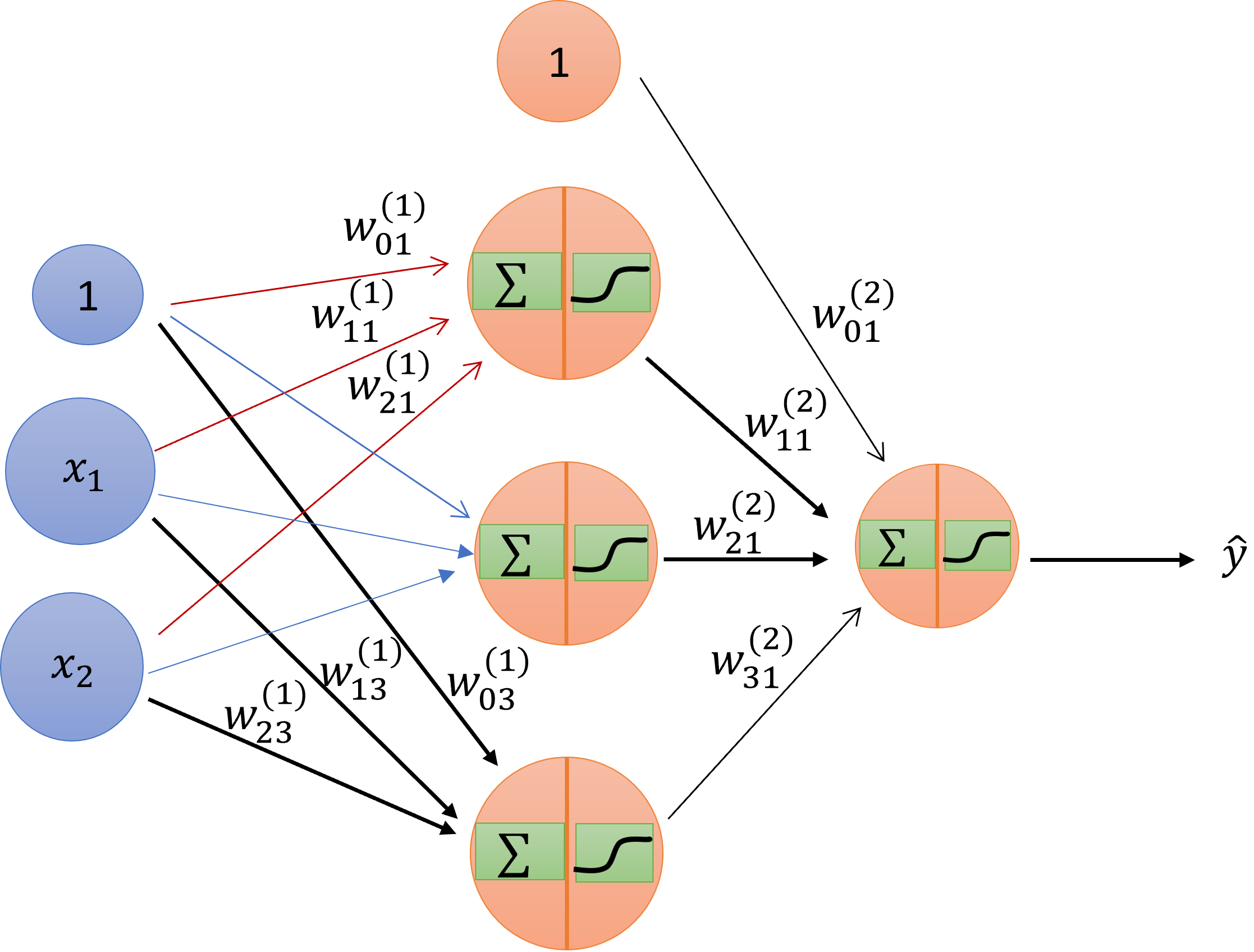
Fig.1. Schematic drawing of a 2 layer neuron networks

First, we use Fig. 1 to introduce some notations. The input-output relation can be expressed in matrix format:

\[ \left[ x^{(2)}_1, x^{(2)}_2, x^{(2)}_3 \right] = \left[ 1, x^{(1)}_1, x^{(1)}_2 \right] \begin{bmatrix} w^{(1)}_{01}, & w^{(1)}_{02}, & w^{(1)}_{03} \\ w^{(1)}_{11}, & w^{(1)}_{12}, & w^{(1)}_{13} \\ w^{(1)}_{21}, & w^{(1)}_{22}, & w^{(1)}_{23} \end{bmatrix} \]

In general,

\[ w^{(l)}_{ij} \begin{cases} 1 \le l \le L & layers \\ 0 \le i \le d^{(l-1)} & inputs \\ 1 \le j \le d^{(l)} & outputs \end{cases} \]

\[ x_j^{(l)} = \theta(s_j^{(l)}) = \theta(\sum_{i=0}^{d^{(l-1)}}w_{ij}^{(l)}x_i^{(l-1)}) \]

Here \(\theta\) is the activation function.

Optimizer

Let us see how we can optimize the weights \(w_{ij}^{(l)}\). Assume \(e(W)\) is the cost function.

\[ \begin{align} \frac{\partial e(W)}{\partial w^{(l)}_{ij}} & = \frac{\partial e(W)}{\partial s^{(l)}_{j}}\times\frac{\partial s^{(l)}_{j}}{\partial w^{(l)}_{ij}} \\ & = \delta^{(l)}_j \times x_i^{(l-1)} \end{align} \]

\[ \delta^{(L)}_1 = \frac{\partial e(W)}{\partial s^{(L)}_{1}} = \frac{\partial e(W)}{\partial\theta}\frac{\partial\theta}{\partial s^{(L)}_{1}} = \frac{\partial e(W)}{\partial\theta} \theta'(s^{(L)}_{1}) \]

Back propagation of \(\delta\)

\[ \begin{align} \delta^{(l-1)}_i & = \frac{\partial e(W)}{\partial s^{(l-1)}_{i}} \\ & = \sum_{j=1}^{d^{(l)}}\frac{\partial e(W)}{\partial s^{(l)}_{j}}\frac{\partial s^{(l)}_{j}}{\partial x^{(l-1)}_{i}} \frac{\partial x^{(l-1)}_{i}}{\partial s^{(l-1)}_{i}} \\ & = \sum_{j=1}^{d^{(l)}} \delta^{(l)}_j \times w_{ij}^{(l)} \times \theta'(s^{(l-1)}_{i}) \\ & = \theta'(s^{(l-1)}_{i}) \sum_{j=1}^{d^{(l)}}w_{ij}^{(l)} \delta^{(l)}_j \end{align} \]

The algorithm

Initialize all weights \(w_{ij}^{(l)}\) at random
for t = 0, 1, 2, , do
Pick \(n \in {1, 2, \cdots, N}\)
Forward: Compute all \(x_j^{(l)}\)
Backward: Compute all \(\delta_j^{(l)}\)
Update the weights: \(w_{ij}^{(l)} \leftarrow w_{ij}^{(l)} - \eta x_i^{(l-1)}\delta_j^{(l)}\)
Iterate to the next step until it is time to stop
Return the final weights \(w_{ij}^{(l)}\)

Some activation functions

Let us define two activation functions and their derivatives. The sigmoid function

\[ \sigma(x) = \frac{1}{1+e^{-x}} \] and its derivative

\[ \sigma'(x) = \sigma(x) (1 - \sigma(x)) \]

sigmoid = function(x) {
  y = list()
  sigma_x <- 1 / (1 + exp(-x))
  y[[1]] <- sigma_x
  y[[2]] <- sigma_x * (1 - sigma_x)
  return(y)
}

x <- seq(-5, 5, 0.01)
plot(x, sigmoid(x)[[1]])
lines(x, sigmoid(x)[[2]], col=2)
legend("topleft", legend = c("Sigmoid", "Derivative"),col = c(1,2), bty='n', lty = 1, cex = 0.8)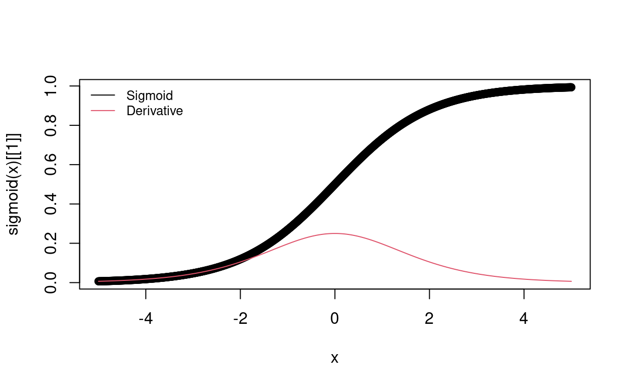

relu <- function(x){
  y <- list()
  y[[1]] <- ifelse(x < 0, 0, x)
  y[[2]] <- ifelse(x < 0, 0, 1)
  return(y)
}
plot(x, relu(x)[[1]])
lines(x, relu(x)[[2]], col=2)
legend("topleft", legend = c("Relu", "Derivative"),col = c(1,2), bty='n', lty = 1, cex = 0.8)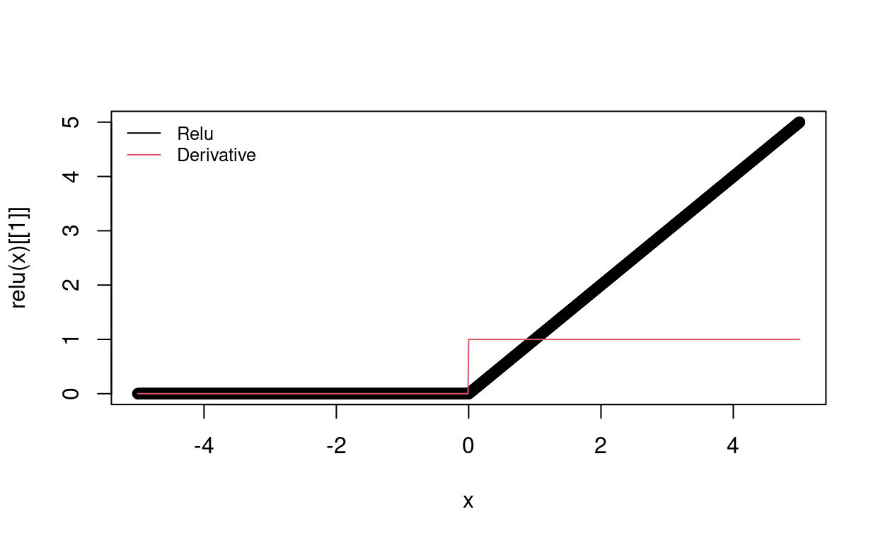

The cost function

# compare Ypredicted with Yreal.
cost <- function(Yp, Yr) {
  y <- list()
  y[[1]] <- mean((Yp -Yr)^2)
  y[[2]] <- (Yp - Yr)
  return(y)
}

Implementation

We shall again use the simple NAND (not-and) gate model to implement the algorithm step by step. The sample has two features. The samples are (0, 0), (0, 1), (1, 0), and (1, 1). The corresponding outputs are 1, 1, 1, 0. They can be expressed in matrix:

\[ X = \begin{bmatrix} 0 & 0 \\ 0 & 1 \\ 1 & 0 \\ 1 & 1 \end{bmatrix} \] \[ Y = \begin{bmatrix} 1 \\ 1 \\ 1 \\ 0 \end{bmatrix} \]

Create the data

X <- matrix(c(0, 0, 1, 1, 0, 1, 0, 1), ncol = 2)
Y <- c(1, 1, 1, 0)

Create the model template using R6 class. “<<-” means global variables.

neurona <- setRefClass(
  "neurona",
  fields = list(
    # activation function
    fun_act = "list",
    num_connections = "numeric",
    num_neurons = "numeric",
    W = "matrix",
    b = "numeric"
  ),
  methods = list(
    initialize = function(fun_act, num_connections, num_neurons){
      fun_act <<- fun_act
      num_connections <<- num_connections
      num_neurons <<- num_neurons
      W <<- matrix(runif(num_connections * num_neurons), nrow = num_connections)
      b <<- runif(num_neurons)
    }
  )
)

Create a 2-layer models.

set.seed(123456)
# number of neurons in the first layer == number of features
n = ncol(X)
# number of neurons at each layer
neurons = c(n, 3, 1)  
# activation function at each layer
functions = list(sigmoid, relu) 
# a global variable
net <- list()

for (i in 1:(length(neurons)-1)) {
  net[[i]] <- neurona$new(functions[i], neurons[i], neurons[i+1])
}

Forward: Compute all \(x_j^{l}\)

# compute all x
# net is global
Forward <- function(x) {
  out = list()
  # each element has two parts: s and \theta(s)
  out[[1]] <- append(list(matrix(0, ncol = 2, nrow = 1)), list(x))
  
  for (i in 1:length(net)) {
    # sum 
    z = list((out[[length(out)]][[2]] %*% net[[i]]$W + net[[i]]$b))
    # applying activation function
    a = list(net[[i]]$fun_act[[1]](z[[1]])[[1]])
    out[[i + 1]] <- append(z, a)
  }
  return(out)
}

out <- Forward(X[1,,drop=FALSE])
out

## [[1]]
## [[1]][[1]]
##      [,1] [,2]
## [1,]    0    0
## 
## [[1]][[2]]
##      [,1] [,2]
## [1,]    0    0
## 
## 
## [[2]]
## [[2]][[1]]
##          [,1]       [,2]      [,3]
## [1,] 0.534858 0.09652624 0.9878469
## 
## [[2]][[2]]
##           [,1]      [,2]      [,3]
## [1,] 0.6306154 0.5241128 0.7286624
## 
## 
## [[3]]
## [[3]][[1]]
##          [,1]
## [1,] 1.861894
## 
## [[3]][[2]]
##          [,1]
## [1,] 1.861894

Backward: Compute all \(\delta^{(l)}_j\)

# compute all delta
Backward <- function(out, cost, Yr) {
delta <- list()

for (i in rev(1:length(net))) {
  z = out[[i+1]][[1]]
  a = out[[i+1]][[2]]
  
  if (i == length(net)) {
    delta[[1]] <- cost(a, Yr)[[2]] * net[[i]]$fun_act[[1]](z)[[2]]
  } else {
    # delta[[1]] dynamically point to the first one in the list delta
    delta <- c(list(delta[[1]] %*% t(net[[i+1]]$W) * net[[i]]$fun_act[[1]](z)[[2]]), delta)
  }
}
return(delta)
}

delta <- Backward(out, cost, Y[1])
delta

## [[1]]
##            [,1]      [,2]      [,3]
## [1,] 0.03364278 0.1715455 0.1011873
## 
## [[2]]
##           [,1]
## [1,] 0.8618937

Update the weights

# Since net is global, do not need return
UpdateW <- function(out, delta, lr = 0.05) {
  for (i in rev(1:length(net))) {
    net[[i]]$b <- net[[i]]$b - delta[[i]][1,] * lr
    net[[i]]$W <- net[[i]]$W - t(out[[i]][[2]]) %*% delta[[i]] * lr
  }
}

net

## [[1]]
## Reference class object of class "neurona"
## Field "fun_act":
## [[1]]
## function(x) {
##   y = list()
##   sigma_x <- 1 / (1 + exp(-x))
##   y[[1]] <- sigma_x
##   y[[2]] <- sigma_x * (1 - sigma_x)
##   return(y)
## }
## <bytecode: 0x557ecfb7a650>
## 
## Field "num_connections":
## [1] 2
## Field "num_neurons":
## [1] 3
## Field "W":
##           [,1]      [,2]      [,3]
## [1,] 0.7977843 0.3912557 0.3612941
## [2,] 0.7535651 0.3415567 0.1983447
## Field "b":
## [1] 0.53485796 0.09652624 0.98784694
## 
## [[2]]
## Reference class object of class "neurona"
## Field "fun_act":
## [[1]]
## function(x){
##   y <- list()
##   y[[1]] <- ifelse(x < 0, 0, x)
##   y[[2]] <- ifelse(x < 0, 0, 1)
##   return(y)
## }
## <bytecode: 0x557eceb18d80>
## 
## Field "num_connections":
## [1] 3
## Field "num_neurons":
## [1] 1
## Field "W":
##           [,1]
## [1,] 0.1675695
## [2,] 0.7979891
## [3,] 0.5937940
## Field "b":
## [1] 0.90531

UpdateW(out, delta, lr = 0.05)
net

## [[1]]
## Reference class object of class "neurona"
## Field "fun_act":
## [[1]]
## function(x) {
##   y = list()
##   sigma_x <- 1 / (1 + exp(-x))
##   y[[1]] <- sigma_x
##   y[[2]] <- sigma_x * (1 - sigma_x)
##   return(y)
## }
## <bytecode: 0x557ecfb7a650>
## 
## Field "num_connections":
## [1] 2
## Field "num_neurons":
## [1] 3
## Field "W":
##           [,1]      [,2]      [,3]
## [1,] 0.7977843 0.3912557 0.3612941
## [2,] 0.7535651 0.3415567 0.1983447
## Field "b":
## [1] 0.53317582 0.08794896 0.98278758
## 
## [[2]]
## Reference class object of class "neurona"
## Field "fun_act":
## [[1]]
## function(x){
##   y <- list()
##   y[[1]] <- ifelse(x < 0, 0, x)
##   y[[2]] <- ifelse(x < 0, 0, 1)
##   return(y)
## }
## <bytecode: 0x557eceb18d80>
## 
## Field "num_connections":
## [1] 3
## Field "num_neurons":
## [1] 1
## Field "W":
##           [,1]
## [1,] 0.1403933
## [2,] 0.7754027
## [3,] 0.5623925
## Field "b":
## [1] 0.8622153

Put together

# train sample by sample
train <- function(xtrain, ytrain, cost, lr=0.01) {
  # compute all x
  out <- Forward(xtrain)
  # compute all delta
  delta <- Backward(out, cost, ytrain)
  # updata weights
  UpdateW(out, delta, lr)
  return(out[[length(out)]][[2]])
}

lr = 0.01
N <- nrow(X)
err_epo <- c()
for (ep in seq(50000)) {
err <- c()
Yp <- c()
for (i in 1:N) {
  # keep matrix format
  xtrain <- X[i,,drop=FALSE]
  ytrain <- Y[i]
  out <- train(xtrain, ytrain, cost, lr)
  err <- append(err, cost(out[1], ytrain)[[1]])
  Yp <- append(Yp, out[1])
} 
err_epo <- append(err_epo, mean(err))
}

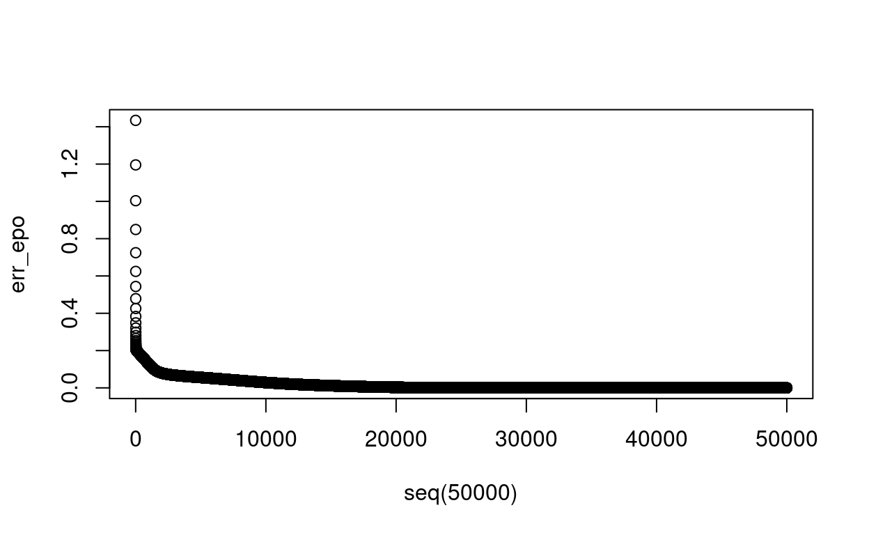
# print out prediction
cat(Yp, '\n')

## 1.000008 0.9999951 0.999995 2.512352e-06

# check convergence
plot(seq(50000), err_epo)