Neural networks from scratch using batch gradient descent with R

Click Start Over menu at the left bottom to start Back to Contents

Notations

\(\mathcal{X}\) space
\(X\) matrix or a random variable
\(\pmb{X}\) operator
\(\pmb{x}\) vector
\(\mathscr{A}\) algorithm

Stochastic gradient descent

Gradient descent (GD) method minimizes an error function with respect to \(\pmb{w}\):

\[ E_{in}(\pmb{w}) = \frac{1}{N}\sum_{n=1}^{N}e(h(\pmb{x}_n), y_n) \]

In order to implement gradient descent, we need to evaluate the hypothesis at every point in our sample to get the error. Then we compute the direction in which we would go

\[ \Delta\pmb{w} = -\eta \nabla E_{in}(\pmb{w}) \]

Indeed, we can get the gradient with respect to that vector and go down the error surface, along the direction suggested by gradient descent. The steps were iterative, and so we take one step at a time. And one step is a full epoch, in the sense that we call something epoch when all the examples are considered at once.

The difference we are going to do now is that, instead of having the movement in the \(\pmb{w}\) space based on all of the examples, we are going to try to do it based on one example at a time. That’s what will make stochastic gradient descent. So because now we are going to have another method, we’re going to label the standard gradient descent as being batch gradient descent. It takes a batch of all the examples and does a move at once.

The stochastic aspect is as follows. We pick one example \((\pmb{x}_n, y_n)\) at a time. Think of it that you pick it at random. We apply GD to \(e(h(\pmb{x}_n), y_n)\), and then get the average

\[ \mathbb{E}[-\nabla e(h(\pmb{x}_n), y_n)] = \frac{1}{N}\sum_{n=1}^{N}-\nabla e(h(\pmb{x}_n), y_n) = -\nabla E_{in} \]

So the expected value is exactly the gradient descent direction. This happens to be identically minus the gradient of the total in-sample error. So it’s as if, at least in expected value, we are actually going along the direction we want, except that we now involve one example in the computation. So we can think that for one example, I’m going along the expected direction plus some noise. So the hope now is that by the time we did it a lot of times, the noise will average out and we actually will be going along the ideal direction. So it’s a randomized version of gradient descent, and it’s called stochastic gradient descent, SGD for short.

Now let’s look at the benefits of having that stochastic aspect. The main benefit by far that is the motivation for having this is that it’s a cheaper computation. Think of one step that we’re going to do using stochastic gradient descent. We take one example, we put the input and get the output, and then compute whatever the gradient is for the example. If we’re doing the batch gradient descent, you will do this for all the examples before we can declare a single move. Nevertheless, the expected value of SGD move in the cheaper version is the same as the other one in GD.

The second advantage is randomization. There is an aspect of optimization that makes randomization advantageous. In general, and in neural networks for sure, we are going to get lots of hills and valleys in your error surface. So depending on where we start, we may end up in one local minimum or another. We may not get the best one. Because according to gradient descent, as long as the gradient is zero, we stop there. So randomization would help choose random start points and go in random different directions. So there is a chance that we may escape from the local minima.

In another situation, we could be having the surface being very, very flat and then finally going down. Gradient descent tells us it is OK to terminate on the flat surface because the gradient is zero. Every now and then when we do the random things, the fluctuation might take us further down the flat surface.

The third advantage is that it’s very simple. It is the simplest possible optimization we can think of. We take one example, we do something, and we’re ready to go.

Neural networks

Let’s start with the biological inspiration of neural networks, because it’s an important factor. That’s where they got their name. Biological inspiration is a method we have really used in engineering applications a number of times. We are interested in replicating the biological function. You know, this is the humans learning. Now we want machines to learn. So in order to replicate the function, our first order is to replicate the structure. So in the case of neural networks, this is the biological system.

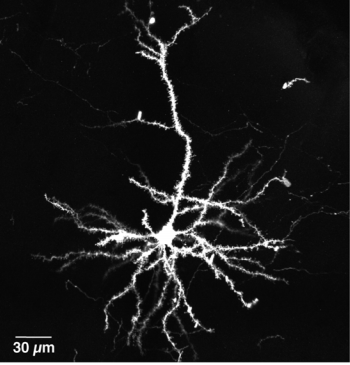
Scanning electron microscopy of a single neuron. Hirabayashi, et al.

We have neurons connected by synapses, there are a large number of them. Each of them does a simple job. The job, the action of a particular neuron, depends on the stimuli coming from different synapses. Synapses have weights. To achieve the intelligence or the learning that a biological system does, articifical neural networks are designed. The neural network will look like this:

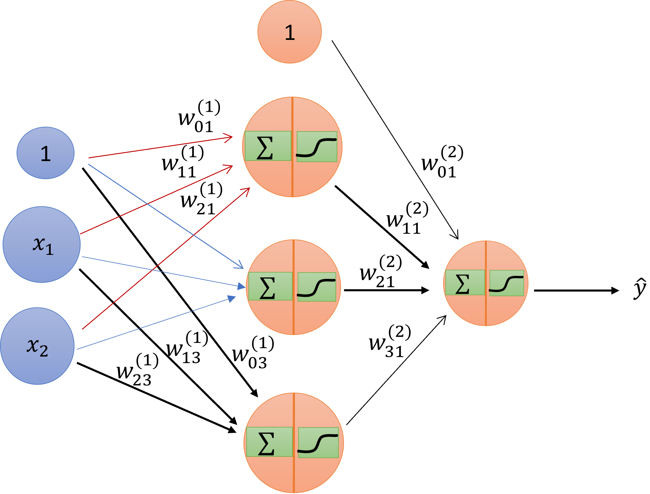
Schematic drawing of an artificial neural network.

It has the inputs– same as inputs before– and it has layers. And each layer has a nonlinearity. I’m referring to the nonlinearity generically as theta.

The first column is the input \(\pmb{x}\). So you are going to apply your input \(\pmb{x}\) from an actual example to this, follow the rules of derivation from one layer to another until you arrive at the end, and then you are going to declare at the end that this is the value of my hypothesis, the neural-network hypothesis, on that \(\pmb{x}\). The intermediate values we are going to call hidden layers, because the user doesn’t see them. You put the input, there’s a black box, and then comes output. If you open the box, you’ll find that there are layers. For a notation, we’re going to consider that we have \(L\) layers. So in this case, it will be three layers. The first layer is the input layer; the second is one hidden layer; the third is the output layer.

First thing, I’m going to define the nonlinearity that I described. It’s a soft threshold and we are going to use the \(tanh\), the hyperbolic tangent:

\[ \theta(s) = tanh(s) = \frac{e^s - e^{-s}}{e^s + e^{-s}} \]

The benefit of this function is analytic and very well-behaved for the optimization. Now I’m going to introduce to you the notation of the neural network.

\[ w^{(l)}_{ij} \begin{cases} 1 \le l \le L & layers \\ 0 \le i \le d^{(l-1)} & inputs \\ 1 \le j \le d^{(l)} & outputs \end{cases} \]

Now, let’s see the function that is being implemented.

\[ x_j^{(l)} = \theta(s_j^{(l)}) = \theta(\sum_{i=0}^{d^{(l-1)}}w_{ij}^{(l)}x_i^{(l-1)}) \] \[ \begin{align} \frac{\partial e(w)}{\partial w^{(l)}_{ij}} & = \frac{\partial e(w)}{\partial s^{(l)}_{j}}\times\frac{\partial s^{(l)}_{j}}{\partial w^{(l)}_{ij}} \\ & = \delta^{(l)}_j \times x_i^{(l-1)} \end{align} \] \[ \delta^{(L)}_1 = \frac{\partial e(w)}{\partial s^{(L)}_{1}} = \frac{\partial e(w)}{\partial\theta}\frac{\partial\theta}{\partial s^{(L)}_{1}} = \frac{\partial e(w)}{\partial\theta} (1-\theta^2(s)) \]

Back propagation of \(\delta\)

\[ \begin{align} \delta^{(l-1)}_i & = \frac{\partial e(w)}{\partial s^{(l-1)}_{i}} \\ & = \sum_{j=1}^{d^{(l)}}\frac{\partial e(w)}{\partial s^{(l)}_{j}}\frac{\partial s^{(l)}_{j}}{\partial x^{(l-1)}_{i}} \frac{\partial x^{(l-1)}_{i}}{\partial s^{(l-1)}_{i}} \\ & = \sum_{j=1}^{d^{(l)}} \delta^{(l)}_j \times w_{ij}^{(l)} \times \theta'(s^{(l-1)}_{i}) \\ & = \theta'(s^{(l-1)}_{i}) \sum_{j=1}^{d^{(l)}}w_{ij}^{(l)} \delta^{(l)}_j \end{align} \]

The algorithm

Initialize all weights \(w_{ij}^{(l)}\) at random
for t = 0, 1, 2, , do
Pick \(n \in {1, 2, \cdots, N}\)
Forward: Compute all \(x_j^{(l)}\)
Backward: Compute all \(\delta_j^{(l)}\)
Update the weights: \(w_{ij}^{(l)} \leftarrow w_{ij}^{(l)} - \eta x_i^{(l-1)}\delta_j^{(l)}\)
Iterate to the next step until it is time to stop
Return the final weights \(w_{ij}^{(l)}\)

Notes 1. We pick n at random—that’s what makes stochastic gradient descent. There are lots of choices. An epoch is one run. And it’s a good idea to get all the examples. So one way to get it to be random and still guarantee that you get all of them is, instead of choosing the point at random, you choose a random permutation from 1 to N, and then go through that in order. And then for the next epoch, you do another permutation. If you do it this way, eventually every example we will contribute the same, but an epoch will be a little bit more difficult to define. You’re can define it simply as N iterations, regardless of whether you covered all of them or not. That is valid. And some people simply do a sequential version, no randomness at all. You just go through the examples, or you have a fixed permutation, and you go through the examples in that order, and keep repeating it. And there are some observations about differences, but the differences are not that profound.

Notes 2. The final weights depend on the order in which the samples are picked. They will depend on the initial condition. They will depend on the order of presentation. They will depend on that, but that is inherent in the game. We are never assured of getting to the perfect minimum, the global minimum. We will get to a local minimum, and anything will affect us. But the whole idea is that you are going to arrive at a minimum. And if you do what we suggested in the last lecture in the Q&A session, that you just start from different starting points, and have different randomization for the presentation. This randomization could be, you pick a point at random. You could pick a random permutation, and then go through the examples according to that permutation, and then change permutation from epoch to epoch. Or you could simply be lazy and just do it sequentially. And all of these, more or less, get you there– will get you with different results. So if you try a variety of those, let’s say 100 tries, and then pick the best minimum you have, you will get a pretty decent minimum, and will be fairly more robust in terms of independence of the particular choices that you made in any of the 100 cases.

Notes 3. There’s something specific here that I want to emphasize, which is the initialization. Because it’s very tempting to initialize weights to 0, which worked actually very well with logistic regression. If you initialize weights to 0 here, bad things will happen. So let me describe why. First, the prescription is to initialize them at random. Why is initializing 0 bad? If you follow the math, you realize that if I have all the weights being 0, which is what that means, and you have multiple layers, then either the x’s or the delta’s will be 0. In every possible weight, one of the two guys that are sandwiching it will be 0. And therefore, the adjustment of the weight according to your criterion would be 0. And therefore, nothing will happen. This is just because of the terrible coincidence that you are perfectly at the top of a hill, unable to break the symmetry. So you’re not moving. So we introduce randomness: Choose weights that are small and random, and you will be OK.

Implementation

We first use the simple NAND model to implement the NN.

Data

X <- matrix(c(0, 0, 1, 1, 0, 1, 0, 1), ncol = 2)
Y <- matrix(c(1, 1, 1, 0), ncol = 1)

Define loss function

coste <- function(Yp,Yr){
  y <- list()
  y[[1]] <- mean((Yp-Yr)^2)
  y[[2]] <- (Yp-Yr)
  return(y)
}

Create the NN model template.

neurona <- setRefClass(
  "neurona",
  fields = list(
    fun_act = "list",
    numero_conexiones = "numeric",
    numero_neuronas = "numeric",
    W = "matrix",
    b = "numeric"
  ),
  methods = list(
    initialize = function(fun_act, numero_conexiones, numero_neuronas)
    {
      fun_act <<- fun_act
      numero_conexiones <<- numero_conexiones
      numero_neuronas <<- numero_neuronas
      W <<- matrix(runif(numero_conexiones*numero_neuronas),
                   nrow = numero_conexiones)
      b <<- runif(numero_neuronas)
    }
  )
)

Define activation functions

sigmoid = function(x) {
  y = list() 
  sigma_x <- 1 / (1 + exp(-x))
  y[[1]] <- sigma_x
  y[[2]] <- sigma_x * (1 - sigma_x)
  return(y)
}

x <- seq(-5, 5, 0.01)
plot(x, sigmoid(x)[[1]], col='blue')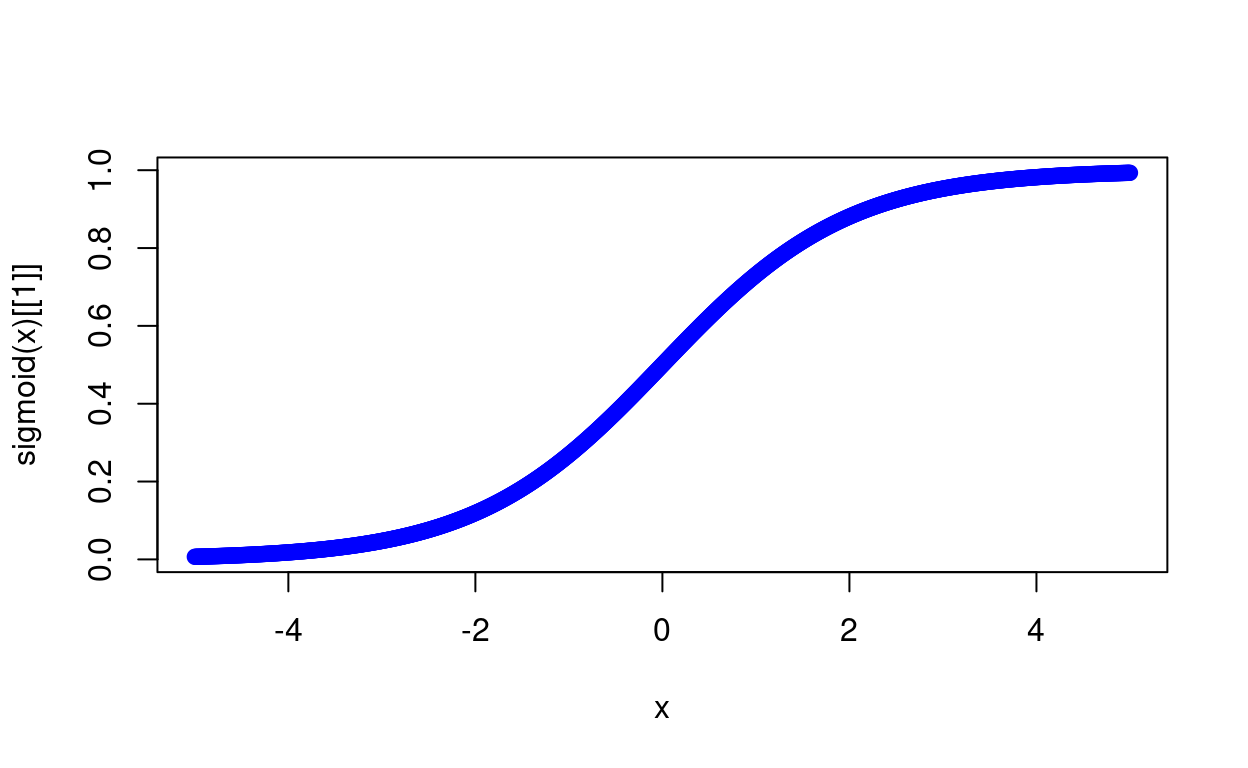

relu <- function(x){
  y <- list()
  y[[1]] <- ifelse(x<0,0,x)
  y[[2]] <- ifelse(x<0,0,1)
  return(y)
}

plot(x, relu(x)[[1]], col='blue')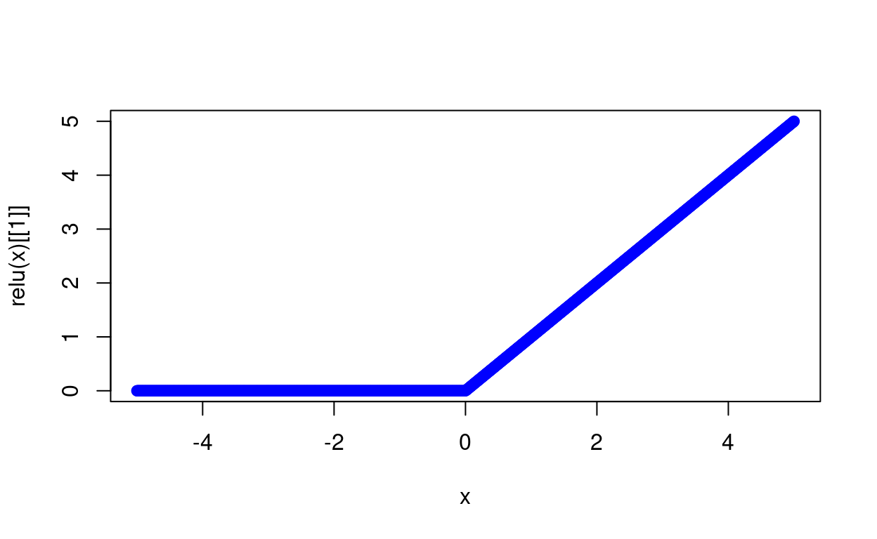

Create NN models

set.seed(123456)
n = ncol(X) #Núm de neuronas en la primera capa
capas = c(n, 3, 1) # Número de neuronas en cada capa.
funciones = list(sigmoid, relu) # Función de activación en cada capa

red <- list()

for (i in 1:(length(capas)-1)){
    red[[i]] <- neurona$new(funciones[i],capas[i], capas[i+1])
}

red

## [[1]]
## Reference class object of class "neurona"
## Field "fun_act":
## [[1]]
## function(x) {
##   y = list() 
##   sigma_x <- 1 / (1 + exp(-x))
##   y[[1]] <- sigma_x
##   y[[2]] <- sigma_x * (1 - sigma_x)
##   return(y)
## }
## 
## Field "numero_conexiones":
## [1] 2
## Field "numero_neuronas":
## [1] 3
## Field "W":
##           [,1]      [,2]      [,3]
## [1,] 0.7977843 0.3912557 0.3612941
## [2,] 0.7535651 0.3415567 0.1983447
## Field "b":
## [1] 0.53485796 0.09652624 0.98784694
## 
## [[2]]
## Reference class object of class "neurona"
## Field "fun_act":
## [[1]]
## function(x){
##   y <- list()
##   y[[1]] <- ifelse(x<0,0,x)
##   y[[2]] <- ifelse(x<0,0,1)
##   return(y)
## }
## 
## Field "numero_conexiones":
## [1] 3
## Field "numero_neuronas":
## [1] 1
## Field "W":
##           [,1]
## [1,] 0.1675695
## [2,] 0.7979891
## [3,] 0.5937940
## Field "b":
## [1] 0.90531

Verify forward in computing all output \(x_{i}^{l}\)

entrenar <- function(red, X,Y, coste){

out = list()
out[[1]] <- append(list(matrix(0,ncol=2,nrow=1)), list(X))

  for(i in c(1:(length(red)))){
    z = list((out[[length(out)]][[2]] %*% red[[i]]$W + red[[i]]$b))
    a = list(red[[i]]$fun_act[[1]](z[[1]])[[1]])
    out[[i+1]] <- append(z,a)
  }
return(out)
}
#rm(a,out,z,i)

out <- entrenar(red, X,Y, coste)
head(out[[2]][[2]])

##           [,1]      [,2]      [,3]
## [1,] 0.6306154 0.5241128 0.7286624
## [2,] 0.7005863 0.7907420 0.6755077
## [3,] 0.8563908 0.7162862 0.6124970
## [4,] 0.8895554 0.6962151 0.8245503

Verify backward in computing all \(\delta^{(l)}_{j}\)

delta <- list()
for (i in rev(1:length(red))){
  z = out[[i+1]][[1]]
  a = out[[i+1]][[2]]

  if(i == length(red)){
    delta[[1]] <- coste(a,Y)[[2]] * red[[i]]$fun_act[[1]](z)[[2]]
  } else{
    delta <- c(list(delta[[1]] %*% t(red[[i+1]]$W) * red[[i]]$fun_act[[1]](z)[[2]]), delta)
  }
}

backprop <- function(out, red, lr = 0.05){

  delta <- list() 

  for (i in rev(1:length(red))){
    z = out[[i+1]][[1]]
    a = out[[i+1]][[2]]

    if(i == length(red)){
      delta[[1]] <- coste(a,Y)[[2]] * red[[i]]$fun_act[[1]](z)[[2]]
    } else{
      delta <- c(list(delta[[1]] %*% W_temp * red[[i]]$fun_act[[1]](z)[[2]]), delta)
    }

    W_temp = t(red[[i]]$W)

    red[[i]]$b <- red[[i]]$b - mean(delta[[1]]) * lr
    red[[i]]$W <- red[[i]]$W - t(out[[i]][[2]]) %*% delta[[1]] * lr
  }
  x = list()
  x[[1]] <- red
  x[[2]] <- out[[length(out)]][[1]]
  return(x)

}

Put all together

red_neuronal <- function(red, X,Y, coste,lr = 0.05){
## Front Prop
out = list()
out[[1]] <- append(list(matrix(0,ncol=2,nrow=1)), list(X))

  for(i in c(1:(length(red)))){
    # sweep(matrix, 2:row, vector, "+"): add vector to all rows
    z = list(sweep(out[[length(out)]][[2]] %*% red[[i]]$W, 2, red[[i]]$b, "+"))
    a = list(red[[i]]$fun_act[[1]](z[[1]])[[1]])
    out[[i+1]] <- append(z,a)
  }


## Backprop & Batch Gradient Descent
delta <- list() 
# loop each layer
for (i in rev(1:length(red))){
  z = out[[i+1]][[1]]
  a = out[[i+1]][[2]]

  if(i == length(red)){
    delta[[1]] <- coste(a,Y)[[2]] * red[[i]]$fun_act[[1]](z)[[2]]
  } else{
    delta <- c(list(delta[[1]] %*% W_temp * red[[i]]$fun_act[[1]](z)[[2]]), delta)
  }

  W_temp = t(red[[i]]$W)

  red[[i]]$b <- red[[i]]$b - colSums(delta[[1]]) * lr
  red[[i]]$W <- red[[i]]$W - t(out[[i]][[2]]) %*% delta[[1]] * lr

}
return(out[[length(out)]][[2]])

}

Test

resultado <- red_neuronal(red, X,Y, coste)
dim(resultado)

## [1] 4 1

for(i in seq(10000)){

  Yt = red_neuronal(red, X,Y, coste, lr=0.01)

  if(i %% 25 == 0){
    if(i == 25){
      iteracion <- i
      error <- coste(Yt,Y)[[1]]
    }else{
          iteracion <- c(iteracion,i)
          error <- c(error,coste(Yt,Y)[[1]])      
    }
  }
}
Yt

##           [,1]
## [1,] 1.2084043
## [2,] 0.8306277
## [3,] 0.8323146
## [4,] 0.1291144

library(ggplot2)

grafico = data.frame(Iteracion = iteracion,Error = error)

ggplot(grafico,aes(iteracion, error)) + geom_line() + theme_minimal() +
  labs(title = "Evolution of the neural network error")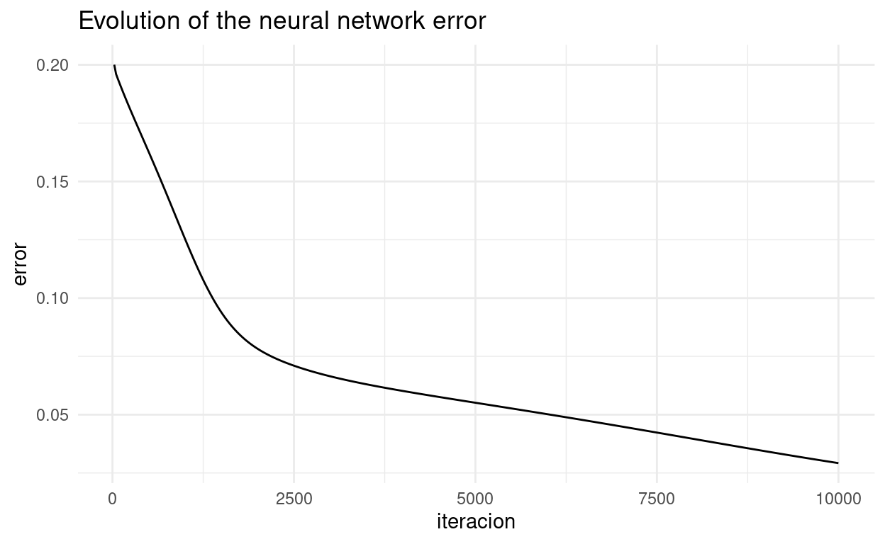

Validation

Data

circulo <- function(x, R, centroX=0, centroY=0){
r = R * sqrt(runif(x))
theta = runif(x) * 2 * pi
x = centroX + r * cos(theta)
y = centroY + r * sin(theta)

z = data.frame(x = x, y = y)
return(z)
}

datos1 <- circulo(150,0.5)
datos2 <- circulo(150,1.5)

datos1$Y <- 1
datos2$Y <- 0
datos <- rbind(datos1,datos2)

rm(datos1,datos2, circulo)

library(ggplot2)
ggplot(datos,aes(x,y, col = as.factor(Y))) + geom_point()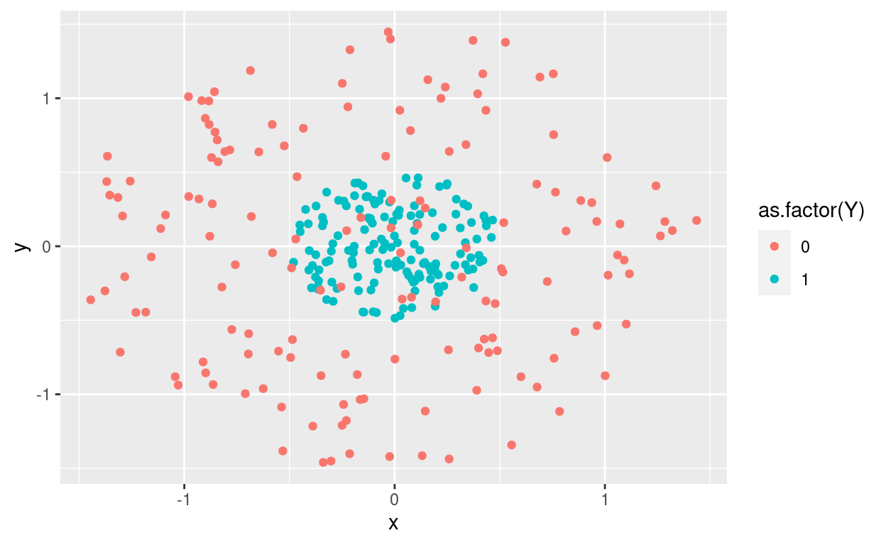

X <- as.matrix(datos[,1:2])
Y <- as.matrix(datos[,3])
rm(datos)

Create NN models

n = ncol(X) # number of samples
capas = c(n, 4, 8, 1) # number of neurons at each layer
funciones = list(sigmoid, relu, sigmoid) # activation function at each layer

red <- list()

for (i in 1:(length(capas)-1)){
    red[[i]] <- neurona$new(funciones[i],capas[i], capas[i+1])
}

red

## [[1]]
## Reference class object of class "neurona"
## Field "fun_act":
## [[1]]
## function(x) {
##   y = list() 
##   sigma_x <- 1 / (1 + exp(-x))
##   y[[1]] <- sigma_x
##   y[[2]] <- sigma_x * (1 - sigma_x)
##   return(y)
## }
## <bytecode: 0x557a5bd7c508>
## 
## Field "numero_conexiones":
## [1] 2
## Field "numero_neuronas":
## [1] 4
## Field "W":
##           [,1]      [,2]      [,3]         [,4]
## [1,] 0.1596998 0.0371191 0.7992258 4.358472e-01
## [2,] 0.2993877 0.8459795 0.3389163 8.299761e-05
## Field "b":
## [1] 0.3220118 0.2846790 0.1041439 0.9212897
## 
## [[2]]
## Reference class object of class "neurona"
## Field "fun_act":
## [[1]]
## function(x){
##   y <- list()
##   y[[1]] <- ifelse(x<0,0,x)
##   y[[2]] <- ifelse(x<0,0,1)
##   return(y)
## }
## <bytecode: 0x557a5ab86408>
## 
## Field "numero_conexiones":
## [1] 4
## Field "numero_neuronas":
## [1] 8
## Field "W":
##             [,1]      [,2]       [,3]      [,4]      [,5]       [,6]      [,7]
## [1,] 0.006928717 0.6922922 0.86005834 0.9308268 0.9148424 0.42066158 0.4465478
## [2,] 0.761530815 0.6346438 0.94428447 0.8792403 0.3988850 0.07305766 0.1024712
## [3,] 0.009982344 0.9669701 0.51379921 0.3091294 0.9162152 0.53495507 0.8157699
## [4,] 0.102126769 0.7660100 0.02357673 0.6642692 0.5391597 0.83908358 0.9408199
##           [,8]
## [1,] 0.3988609
## [2,] 0.2848591
## [3,] 0.4890111
## [4,] 0.9287517
## Field "b":
## [1] 0.87457192 0.82278084 0.79335961 0.11796003 0.01810510 0.73025046 0.49823996
## [8] 0.03566021
## 
## [[3]]
## Reference class object of class "neurona"
## Field "fun_act":
## [[1]]
## function(x) {
##   y = list() 
##   sigma_x <- 1 / (1 + exp(-x))
##   y[[1]] <- sigma_x
##   y[[2]] <- sigma_x * (1 - sigma_x)
##   return(y)
## }
## <bytecode: 0x557a5bd7c508>
## 
## Field "numero_conexiones":
## [1] 8
## Field "numero_neuronas":
## [1] 1
## Field "W":
##           [,1]
## [1,] 0.1251371
## [2,] 0.8089088
## [3,] 0.9232700
## [4,] 0.4659551
## [5,] 0.9014398
## [6,] 0.1539973
## [7,] 0.4071012
## [8,] 0.6166067
## Field "b":
## [1] 0.4227565

Train

for(i in seq(10000)){

  Yt = red_neuronal(red, X,Y, coste, lr=0.01)

  if(i %% 25 == 0){
    if(i == 25){
      iteracion <- i
      error <- coste(Yt,Y)[[1]]
    }else{
          iteracion <- c(iteracion,i)
          error <- c(error,coste(Yt,Y)[[1]])      
    }
  }
}

Check

library(ggplot2)

grafico = data.frame(Iteracion = iteracion,Error = error)

ggplot(grafico,aes(iteracion, error)) + geom_line() + theme_minimal() +
  labs(title = "Evolution of the neural network error")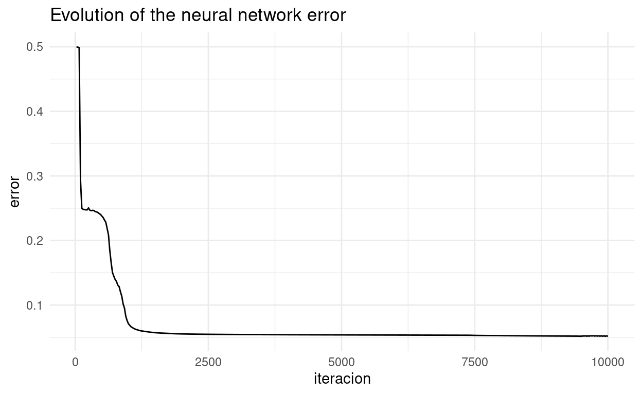

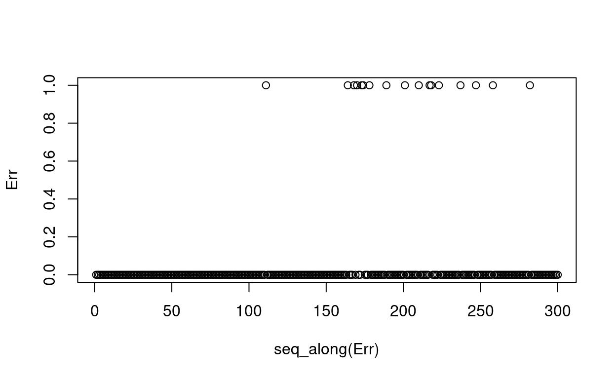
Yt <- ifelse(Yt < 0.5, 0, 1)
Err <- abs(Yt -Y)
plot(seq_along(Err), Err)

References

https://www.youtube.com/watch?v=Ih5Mr93E-2c&list=PLvx5ei9aEEqKgDZ7oaQGSToFi-QER4v1M&index=11

https://anderfernandez.com/en/blog/how-to-code-a-neural-network-from-scratch-in-r/