Click Start Over menu at the left bottom to start Back to Contents
Notations
\(\mathcal{X}\) space
\(X\) matrix
\(\pmb{X}\) operator
\(\pmb{x}\) vector
\(\mathscr{A}\) algorithm
When ML is used?
There is a pattern to be discovered
We cannot describe underlying process/phenomena using mathematical equations/formula
Data available
What is the basic components of ML?
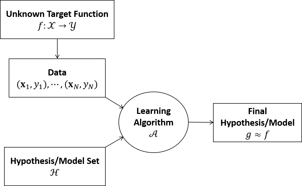
Fig.1. The scheme of machine learning.
Input \(\pmb{x}\) (e.g. customer’s info)
Output \(y\) (e.g. yes/no)
Target function: \(f: \mathcal{X} \rightarrow \mathcal{Y}\) (unknown, this is what we want to learn from data.)
Data: \((\pmb{x}_1, y_1), \cdots, (\pmb{x}_N, y_N)\) (historial records)
Hyperthesis/models: an approximation to the target function: \(g: \mathcal{X} \rightarrow \mathcal{Y}\) (things to learn, formula/models to be delivered)
The goal of machine learning is to find the best \(g\) to approximate \(f\).
Basic premise of learning
using a set of observations to uncover the underlying process.
supervised learning: labels given
unsupervised learning: no labels given
reinforcement learning: feedback, some output, grade for output
Perceptron — the simplest model
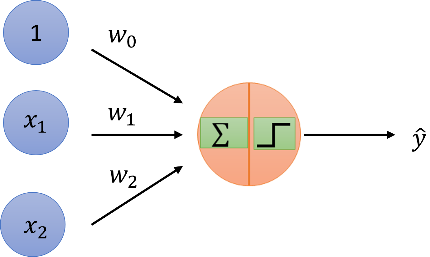
Fig.2. Schematic drawing of a single layer perceptron.
The problem
For input \(\pmb{x}=(x_1, \cdots, x_d)\), attributes/features of a customer, approve credit if \[\sum_{i=1}^d w_i x_i > threshold\]
The hypothesis
This linear formula \(h \in \mathcal{H}\) can be written as
\[ h(\pmb{x}) = sign\left(\left(\sum_{i=1}^d w_i x_i\right)-threshold\right) \] We want to learn the parameters \(w_1, \cdots, w_d\) and \(w_0 = -threshold\).
Introducing an artificial coordinates \(x_0 =1\),
\[ h(\pmb{x}) = sign\left(\sum_{i=0}^d w_i x_i\right) = sign(\pmb{w}^T \pmb{x}) \]
Perceptron learning algorithm (PLA)
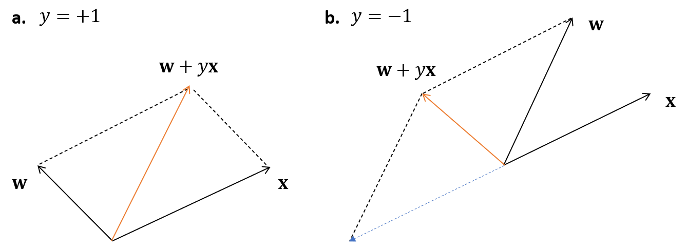
Given the training set: \((\pmb{x}_1, y_1), (\pmb{x}_2, y_2), \cdots, (\pmb{x}_N, y_N)\), pick a misclassified point: \(sign(\pmb{w}^T \pmb{x}_n) \not= y_n\), and update the weight vector: \[ \pmb{w} \leftarrow \pmb{w} + y_n \pmb{x}_n \] interaction \(t=1, 2, 3, \cdots\), pick a misclassified point from training data and run a PLA iteration on it.
code
Let us start with a simple example, the NAND (not-and) gate which outputs false only if all inputs are true. To match the above hypothesis, we denote false by -1 and true by 1.
The inputs after prepending \(x_0 = 1\):
\[ \begin{array}{ccc} \;\;\;\;\;\;x_{i0} & x_{i1} & x_{i2} \end{array} \\ \begin{array}{c} \pmb{x}_1 \\ \pmb{x}_2 \\ \pmb{x}_3 \\ \pmb{x}_4 \end{array} \left( \begin{array}{ccc} 1 & 0 & 0 \\ 1 & 0 & 1 \\ 1 & 1 & 0 \\ 1 & 1 & 1 \\ \end{array} \right) \]
The outputs
\[ \begin{array}{c} y_1 \\ y_2 \\ y_3 \\ y_4 \end{array} \left( \begin{array}{c} 1 \\ 1 \\ 1 \\ -1 \\ \end{array} \right) \]
- Prepare data
# nrow = number of samples, ncol = number of features
X <- matrix(c(1, 1, 1, 1, 0, 0, 1, 1, 0, 1, 0, 1), nrow = 4)
Y <- c(1, 1, 1, -1)- Formulate the hypotheses
# the length of weights
n.feature <- dim(X)[2]
W <- rep(1, n.feature)
G <- sign(X %*% W)- Update the weights
Since \(Y[4]\) is misclassified, we update \(\pmb{w}\) using \((\pmb{x}_4, y_4)\). Here we introduce a concept called the learning rate 0.5. For misclassified points, \(0.5 * (y_4 - g_4) = \pm 1\), otherwise \(0.5 * (y_4 - g_4) = 0\).
W <- W + 0.5 * (Y[4] - G[4]) * X[4, ]- Iterating the updating process
One complete sweep through the data set is known as an “epoch”.
Perceptron <- function(X, Y, eta=0.5, t=10) {
  # X, matrix, each row is a sample
  # Y, target vector, each element is a label
  # eta, learning rate
  # t, number of iterations
  # initialize the weights, length = number of features
  W <- rep(0, dim(X)[2])
  len.data <- dim(X)[1]
  # record interation times
  n <- 0
  # record prediction
  G <- c()
  Err <- c()
  repeat {
    # for each sample
    for (i in 1:len.data) {
 #     G[i] <- sign(X[i,] %*% W)
      tmp <- X[i,] %*% W
      if (tmp >= 0) {
        G[i] <- 1
      } else {
        G[i] <- 0
      }
      W <- W + eta * (Y[i] - G[i]) * X[i, ]
    }
    n <- n + 1
    Err[n] <- (Y - G) %*% (Y - G)
    if ((n == t) | (Err[n] == 0)) {
      break
    }
  }
  return(list(W=W, G=G, Err=Err))
}- Run
X <- matrix(c(1, 1, 1, 1, 0, 0, 1, 1, 0, 1, 0, 1), nrow = 4)
Y <- c(1, 1, 1, 0)
results <- Perceptron(X, Y, 0.1)
print(results$W)
## [1] 0.2 -0.2 -0.1print(results$G)## [1] 1 1 1 0print(results$Err)## [1] 1 3 3 2 1 0- Validation
6.1 Get data
df <- read.csv("testdata.csv", header = TRUE)6.2 Split the data into train/test sets
# shuffle the data
df.mat <- as.matrix(df)
df.mat <- df.mat[sample(dim(df.mat)[1]),]
# split
n <- as.integer(0.7 * dim(df.mat)[1])
train <- df.mat[1:n,]
test <- df.mat[(n+1):dim(df.mat)[1],]
x_train <- train[,1:3]
y_train <- train[,4]
x_test <- test[,1:3]
y_test <- test[,4]6.3 Train
results <- Perceptron(x_train, y_train, 0.1, 50)
print(results$W)
## X0 X1 X2
## -0.4000000 -0.3270215 0.2864476print(results$Err)## [1] 8 06.4 Test
w.hat <- results$W
y.hat <- x_test %*% w.hat
y_hat <- y.hat
y_hat[y.hat >= 0] <- 1
y_hat[y.hat < 0] <- 0
plot(y_test, y_hat)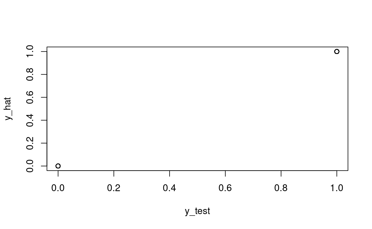
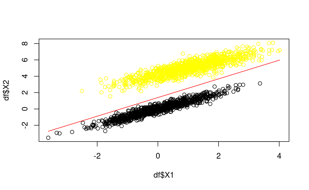
6.5 Plot
xt <- df.mat[,2]
yt <- -(w.hat[1] + w.hat[2] * xt) / w.hat[3]
plot(df$X1, df$X2, col=ifelse(df$X3>0,"yellow","black"))
lines(xt, yt, col="red")