Chapter 1 Linear Modeling: A Least Squares Approach

Click Start Over at the left bottom to start Back to Contents

1.1 The least squares solution

The problem

Given a set of data \((x_{n}, t_{n})_{n=1}^{N}\), we want to find the best model to fit the data from a model pool, for example, the polynomial models:

\[\begin{equation} t = \sum_{k=0}^{K}\omega_{k}x^{k} = \overrightarrow{\omega}^{T}\overrightarrow{x} \label{eq:polynomial} \end{equation}\]

where \[ \overrightarrow{\omega}=\begin{bmatrix} \omega_{0} \\ \omega_{1} \\ \vdots \\ \omega_{K} \end{bmatrix} \qquad \overrightarrow{x}=\begin{bmatrix} 1 \\ x \\ x^2 \\ \vdots \\ x^{K} \end{bmatrix}. \]

In the sense of least squares approach, the best model means we want to find the best values for \(\overrightarrow{\omega}\) to mininize the difference between data and model-based values

\[\begin{equation} \underset{\overrightarrow{\omega}}{\arg\min} \mathcal{L}(\overrightarrow{\omega}) \label{eq:argmin} \end{equation}\]

where \[\begin{equation} \begin{split} \mathcal{L} & = \frac{1}{N}\sum_{1}^{N}(t_n - \overrightarrow{\omega}^{T}\overrightarrow{x_n})^2 \\ & = \frac{1}{N}(\overrightarrow{t}-\textbf{X}\overrightarrow{\omega})^{T}(\overrightarrow{t}-\textbf{X}\overrightarrow{\omega}) \end{split} \label{eq:lossfunc} \end{equation}\]

\[ \overrightarrow{t}=\begin{bmatrix} t_{1} \\ t_{2} \\ \vdots \\ t_{N} \end{bmatrix} \qquad \textbf{X}=\begin{bmatrix} \overrightarrow{x_{1}}^{T} \\ \overrightarrow{x_{2}}^{T} \\ \vdots \\ \overrightarrow{x_{N}}^{T} \end{bmatrix} =\begin{bmatrix} 1 & x_{1} & x_{1}^2 & \dots & x_{1}^K \\ 1 & x_{2} & x_{2}^2 & \dots & x_{2}^K \\ \vdots & \vdots & \vdots & \ddots & \vdots \\ 1 & x_{N} & x_{N}^2 & \dots & x_{N}^K \end{bmatrix} \]

The analytical solution

Using the identities in the following Table 1, we obtain

\[\begin{equation} \frac{\partial \mathcal{L}}{\partial \overrightarrow{\omega}} = \frac{2}{N}\textbf{X}^{T}\textbf{X}\overrightarrow{\omega}- \frac{2}{N}\textbf{X}^{T}\overrightarrow{t} = 0 \label{eq:difflossfunc} \end{equation}\]

or \[\begin{equation} \textbf{X}^{T}\textbf{X}\overrightarrow{\omega} = \textbf{X}^{T}\overrightarrow{t} \label{eq:leastsolution} \end{equation}\]

Table 1: Some useful identities when differentiating with respect to a vector.

\(f(\overrightarrow{\omega})\)	\(\frac{\partial f}{\partial \overrightarrow{\omega}}\)
\(\overrightarrow{\omega}^{T}\overrightarrow{x}\)	\(\overrightarrow{x}\)
\(\overrightarrow{x}^{T}\omega\)	\(\overrightarrow{x}\)
\(\overrightarrow{\omega}^{T}\textbf{C}\overrightarrow{\omega}\)	\(2\textbf{C}\overrightarrow{\omega}\)

The numerical solution

Let us do a numerical simulation using a set of synthetic data. We first generate a set of data from a quadratic function with some noise.

# Number of data points 
N = 100 
# Generate random x values between -5 and 5
# for reproducibility, we set a random seed
set.seed(1234)
x = runif(n=N,min=-5,max=5)

## Define the function and the true parameters
# $t = w_0 + w_1x + w_2x^2$
w_0 = 1
w_1 = -2
w_2 = 0.5

## Define t
t = w_0 + w_1*x + w_2*(x^2)

## Add some noise
t = t + 0.5*rnorm(n=N)

## Plot the data
plot(x, t, main = "")

Figure 1: Synthetic data generated from quadratic polynomial.

One may choose any order polynomial function to fit the data, we use third-order, quadratic, and linear model for comparison. The following codes produce the fitted functions.

# Number of data points 
N = 100 
# Generate random x values between -5 and 5
# for reproducibility, we set a random seed
set.seed(1234)
x = runif(n=N,min=-5,max=5)

## Define the function and the true parameters
# $t = w_0 + w_1x + w_2x^2$
w_0 = 1
w_1 = -2
w_2 = 0.5

## Define t
t = w_0 + w_1*x + w_2*(x^2)

## Add some noise
t = t + 0.5*rnorm(n=N)

## Fit the third-orde, quadratic, and a linear model for comparison
X = matrix(c(x^0, x^1, x^2, x^3), ncol = 4, byrow = FALSE)
for (k in c(1, 2, 3)) {
  if (k == 1){
    linear_w = (solve(t(X[,c(1,2)]) %*% X[,c(1,2)]) %*% t(X[,c(1,2)])) %*% t
  }
  if (k == 2) {
    quad_w = (solve(t(X[, c(1, 2, 3)]) %*% X[, c(1, 2, 3)]) %*% t(X[, c(1, 2, 3)])) %*% t
  }
  if (k == 3) {
    third_w = (solve(t(X) %*% X) %*% t(X)) %*% t
  }
}
cat(paste("\n Linear function: t =",linear_w[1,],"+",linear_w[2,],"x \n"))
cat(paste("\n Quadratic function: t =",quad_w[1,],"+",quad_w[2,],"x +",quad_w[3,],"x^2 \n"))
cat(paste("\n Third-order function: t =",third_w[1,],"+",third_w[2,],"x +",third_w[3,],"x^2", "+", third_w[4,],"x^3 \n"))

Let us plot the fitted results.

# Number of data points 
N = 100 
# Generate random x values between -5 and 5
# for reproducibility, we set a random seed
set.seed(1234)
x = runif(n=N,min=-5,max=5)

## Define the function and the true parameters
# $t = w_0 + w_1x + w_2x^2$
w_0 = 1
w_1 = -2
w_2 = 0.5

## Define t
t = w_0 + w_1*x + w_2*(x^2)

## Add some noise
t = t + 0.5*rnorm(n=N)

## Fit the third-orde, quadratic, and a linear model for comparison
X = matrix(c(x^0, x^1, x^2, x^3), ncol = 4, byrow = FALSE)
for (k in c(1, 2, 3)) {
  if (k == 1){
    linear_w = (solve(t(X[,c(1,2)]) %*% X[,c(1,2)]) %*% t(X[,c(1,2)])) %*% t
  }
  if (k == 2) {
    quad_w = (solve(t(X[, c(1, 2, 3)]) %*% X[, c(1, 2, 3)]) %*% t(X[, c(1, 2, 3)])) %*% t
  }
  if (k == 3) {
    third_w = (solve(t(X) %*% X) %*% t(X)) %*% t
  }
}

## Plot the functions
plotx = seq(from=-5,to=5,by=0.01)
plotX = matrix(c(plotx^0, plotx^1, plotx^2, plotx^3), ncol=4, byrow=FALSE)
plot(x, t, main = "")
points(plotx,plotX %*% third_w, type="l", col="purple")
points(plotx,plotX[, c(1, 2, 3)] %*% quad_w, type="l", col="blue")
points(plotx,plotX[,c(1,2)] %*% linear_w, type="l", col="red")
legend(2.,23,c("Third", "Quadratic","Linear"),lty=c(1, 1,1),lwd=c(2.5, 2.5,2.5), col=c("purple", "blue","red"))

Figure 2: Synthetic data fitting to different models.

The discussion

Quiz

1.2 Cross-Validation

The problem

The goal of data-fitting is to make a model best fit to given data. The goal of machine learning is to make a model not only best fit to given data but also best predict unknown data. Best fitting does not guarantee best prediction. Let us look at an example. Table 2 is the data for the Olympic men’s 100 m winning time from year 1896 to 2012.

Table 2: Olympic men’s 100 m winning time (s).

Year	Time
1896	12.00
1900	11.00
1904	11.00
1906	11.20
1908	10.80
1912	10.80
1920	10.80
1924	10.60
1928	10.80
1932	10.30
1936	10.30
1948	10.30
1952	10.40
1956	10.50
1960	10.20
1964	10.00
1968	9.95
1972	10.14
1976	10.06
1980	10.25
1984	9.99
1988	9.92
1992	9.96
1996	9.84
2000	9.87
2004	9.85
2008	9.69
2012	9.63

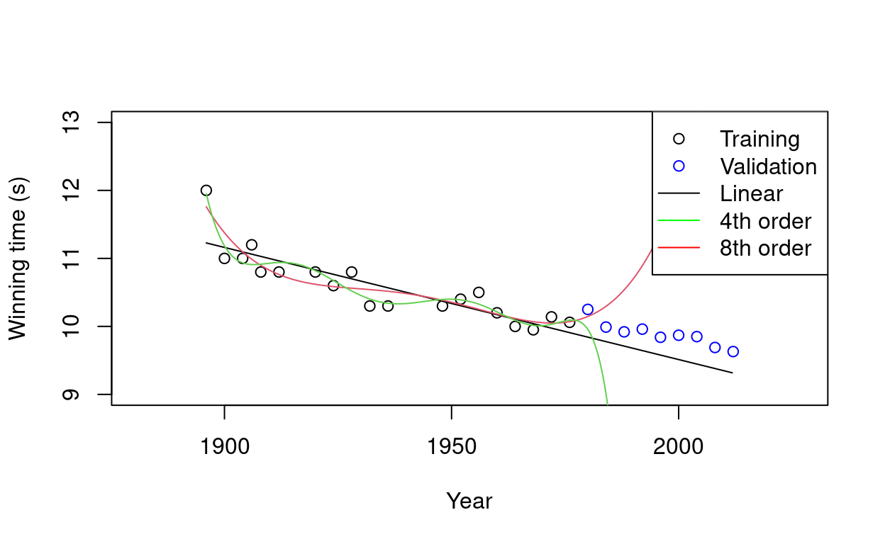
We want to make a model to fit the data before the year 1979 and to predict the winning time after the year 1979. We have chosen the first, fourth and eighth order polynomial as candidate models. Figure 3 shows that the fitting loss (0.058 > 0.03 > 0.017) decreases as orders (1 < 4 < 8) increase. However, the validation loss (0.1 < 7.46 < 16283) has an opposite trend. We say that eighth-order model overfits to the data because it best fits to the data but has worst predictive performance. How can we choose a model that is able to generalize well without over-fitting?

## 
##  Model order: 1, Fitting loss: 0.0581845335803661
##  Model order: 1, Validation loss: 0.101096146346076
##  Model order: 4, Fitting loss: 0.0300995860201469
##  Model order: 4, Validation loss: 7.46538642187292
##  Model order: 8, Fitting loss: 0.0167512675439386
##  Model order: 8, Validation loss: 16283.4732655823

Figure 3: Demonstration of overfitting.

The solution

A popular choice is to use \(K\)-fold cross-validation and repeat the process several times with the data randomly shuffled, allowing averages to be taken across both folds and repetitions. When \(K=N\), it is called leave-one-out cross validation (LOOCV). This scheme is illustrated in the following Figure 4. In this scheme, the data are splitted into \(K\) blocks. \(K-1\) blocks are used for training. One block is used for validation.

Figure 4: Scheme of K-fold.

Let us do a demonstration. We first generate a set of training data, and a set of test data.

# Generate a set of data
# Generate x between -5 and 5
# Generate t from a third order polynomial with some noise
N = 100
set.seed(1234)
x = 10*runif(N) - 5
t = 5*(x^3)  - (x^2) + x + 150*rnorm(length(x))
# generate test data
testx = seq(-5,5,0.01) # Large, independent test set
testt = 5*(testx^3) - (testx^2) + testx + 150*rnorm(length(testx))
plot(x, t, main = "")

Figure 5: Synthetic training and test datasets.

We want to choose the best model from linear to seventh order polynomial models using \(K=10\) fold cross-validation scheme. We split the training data to \(10\) blocks.

N = 100
set.seed(1234)
x = 10*runif(N) - 5
t = 5*(x^3)  - (x^2) + x + 150*rnorm(length(x))
# generate test data
testx = seq(-5,5,0.01) # Large, independent test set
testt = 5*(testx^3) - (testx^2) + testx + 150*rnorm(length(testx))

## Run a cross-validation over model orders
maxorder = 7
X = matrix(x^0, ncol=1)
testX = matrix(testx^0, ncol=1)
K = 10 # K-fold CV
sizes = rep(floor(N/K), K)
## check remaining number
sizes[length(sizes)] = sizes[length(sizes)] + N - sum(sizes)
csizes = c(0,cumsum(sizes))
train_loss <- matrix(nrow=K, ncol=maxorder+1)
cv_loss <- matrix(nrow=K, ncol=maxorder+1)
test_loss <- matrix(nrow=K, ncol=maxorder+1)

We use \(9\) blocks for training and \(1\) block for validation.

N = 100
set.seed(1234)
x = 10*runif(N) - 5
t = 5*(x^3)  - (x^2) + x + 150*rnorm(length(x))
# generate test data
testx = seq(-5,5,0.01) # Large, independent test set
testt = 5*(testx^3) - (testx^2) + testx + 150*rnorm(length(testx))

## Run a cross-validation over model orders
maxorder = 7
X = matrix(x^0, ncol=1)
testX = matrix(testx^0, ncol=1)
K = 10 # K-fold CV
sizes = rep(floor(N/K), K)
## check remaining number
sizes[length(sizes)] = sizes[length(sizes)] + N - sum(sizes)
csizes = c(0,cumsum(sizes))
train_loss <- matrix(nrow=K, ncol=maxorder+1)
cv_loss <- matrix(nrow=K, ncol=maxorder+1)
test_loss <- matrix(nrow=K, ncol=maxorder+1)
# do training, cross-validation and testing
for(k in 0:maxorder){
  if(k >= 1){
    X = cbind(X, x^k)
    testX = cbind(testX, testx^k)
  }
  for(fold in 1:K){
    # Partition the data
    # foldX contains the data for just one fold
    # trainX contains all other data
    foldX = as.matrix(X[(csizes[fold]+1):csizes[fold+1],])
    trainX = X
    trainX = as.matrix(trainX[-((csizes[fold]+1):csizes[fold+1]),])
    foldt = as.matrix(t[(csizes[fold]+1):csizes[fold+1]])
    traint = t
    traint = as.matrix(traint[-((csizes[fold]+1):csizes[fold+1])])
    # training 
    w = solve(t(trainX) %*% trainX) %*% t(trainX) %*% traint
    train_pred = trainX %*% w
    train_loss[fold, k+1] = mean((train_pred - traint)^2)
    # cross-validation
    fold_pred = foldX %*% w
    cv_loss[fold, k+1] = mean((fold_pred-foldt)^2)
    # test
    test_pred = testX %*% w
    test_loss[fold, k+1] = mean((test_pred - testt)^2)
  }
}

Let us have a look at the behaviour of the loss functions.

N = 100
set.seed(1234)
x = 10*runif(N) - 5
t = 5*(x^3)  - (x^2) + x + 150*rnorm(length(x))
# generate test data
testx = seq(-5,5,0.01) # Large, independent test set
testt = 5*(testx^3) - (testx^2) + testx + 150*rnorm(length(testx))

## Run a cross-validation over model orders
maxorder = 7
X = matrix(x^0, ncol=1)
testX = matrix(testx^0, ncol=1)
K = 10 # K-fold CV
sizes = rep(floor(N/K), K)
## check remaining number
sizes[length(sizes)] = sizes[length(sizes)] + N - sum(sizes)
csizes = c(0,cumsum(sizes))
train_loss <- matrix(nrow=K, ncol=maxorder+1)
cv_loss <- matrix(nrow=K, ncol=maxorder+1)
test_loss <- matrix(nrow=K, ncol=maxorder+1)
# do training, cross-validation and testing
for(k in 0:maxorder){
  if(k >= 1){
    X = cbind(X, x^k)
    testX = cbind(testX, testx^k)
  }
  for(fold in 1:K){
    # Partition the data
    # foldX contains the data for just one fold
    # trainX contains all other data
    foldX = as.matrix(X[(csizes[fold]+1):csizes[fold+1],])
    trainX = X
    trainX = as.matrix(trainX[-((csizes[fold]+1):csizes[fold+1]),])
    foldt = as.matrix(t[(csizes[fold]+1):csizes[fold+1]])
    traint = t
    traint = as.matrix(traint[-((csizes[fold]+1):csizes[fold+1])])
    # training 
    w = solve(t(trainX) %*% trainX) %*% t(trainX) %*% traint
    train_pred = trainX %*% w
    train_loss[fold, k+1] = mean((train_pred - traint)^2)
    # cross-validation
    fold_pred = foldX %*% w
    cv_loss[fold, k+1] = mean((fold_pred-foldt)^2)
    # test
    test_pred = testX %*% w
    test_loss[fold, k+1] = mean((test_pred - testt)^2)
  }
}
# plot the loss value for training, cross-validation and testing
par(mfrow=c(1,3))
plot(0:maxorder, colMeans(cv_loss), type="l", xlab="Model Order", ylab="Loss", main="CV Loss", col="blue")
plot(0:maxorder, colMeans(train_loss), type="l", xlab="Model Order", ylab="Loss", main="Train Loss", col="blue")
plot(0:maxorder, colMeans(test_loss), type="l", xlab="Model Order", ylab="Loss", main="Test Loss", col="blue")

Figure 6: The evaluation of loss functions.

From the above Figure 6, we see that the third-order polynomial function is the best model since all the training, cross-validation and testing loss are at the minimum.

The above process can be repeated several times after randomly shuffling the data using the function order <- sample(N)

The discussion

Quiz

1.3 Regularization

The problem

From above discussion, we see that overfitting is due to model complexity. In the polynomial models, model complexity is governed by the coefficients of higher order terms. One way to stop our models becoming too complex is to make the coefficients of higher order terms as small as possible. How can we do that?

The solution

We can impose a penalty on model complexity by minimizing a regularized loss function \(\mathcal{L}'\):

\[\begin{equation} \mathcal{L}' = \mathcal{L} + \lambda \overrightarrow{\omega}^{T} \overrightarrow{\omega} \label{eq:regularized} \end{equation}\]

Following the derivation of Equation (\ref{eq:leastsolution}), we can obtain the regularized least squares solution given by

\[\begin{equation} \overrightarrow{\omega} = (\textbf{X}^{T}\textbf{X} + N \lambda \textbf{I})^{-1} \textbf{X}^{T}\overrightarrow{t} \label{eq:regulsolution} \end{equation}\]

Clearly, if \(\lambda = 0\), we retrieve the original solution. If we increase \(\lambda\), we can see the regularization taking effect. Let us do a demonstration. First we generate a set of synthetic data as shown in Figure 7.

## Generate the data
x = seq(0,1,0.2)
y = (2*x)-3

## Create targets by adding noise
set.seed(1234)
noisevar = 3
t = y + sqrt(noisevar)*rnorm(length(x))

## Plot the data
par(mar = c(5, 4, 4, 10))
plot(x,t,xlab="x",ylab="f(x)", xlim=c(-0.1,1.1),ylim=c(-10,4))

Figure 7: Synthetic data generated by a linear function.

In general, \(N\) data points can be perfectly fitted by an \((N-1)\)th order polynomial. So we choose to fit the 6 data points using a 5th order polynomial.

## Generate the data
x = seq(0,1,0.2)
y = (2*x)-3

## Create targets by adding noise
set.seed(1234)
noisevar = 3
t = y + sqrt(noisevar)*rnorm(length(x))

## Build up the data so that it has up to fifth order terms
testx = seq(0,1,0.01)
X = matrix(x^0)
testX = matrix(testx^0)
for(k in 1:5){
    X = cbind(X,x^k)
    testX = cbind(testX,testx^k)
}
## Plot the data
par(mar = c(5, 4, 4, 10))
plot(x,t,xlab="x",ylab="f(x)",xlim=c(-0.1,1.1),ylim=c(-10,4))
## Fit the model with different values of the regularization parameter
##
# $$\lambda$$
lam = c(0,1e-6,1e-2,1e-1)
for(l in 1:length(lam)){
  lambda = lam[l]
  N = length(x)
  w = solve(t(X)%*%X + N*lambda*diag(dim(X)[2]))%*%t(X)%*%t
  points(testx,testX%*%w,type="l",col=l)
}
par(xpd=T, mar = c(5, 4, 4, 2))
legend(x=1.2,y=-2,legend=c('lambda=0','lambda=10^-6','lambda=10^-2','lambda=10^-1'),
       lty=c(1,1,1,1),col=c("black","red","green","blue"))

Figure 8: The regularization effect.

Figure 8 shows that the model complexity decreases with increasing the regularization parameter \(\lambda\), and better predictive performance can be achieved by varying \(\lambda\). So we can either choose optimal polynomial order (optimal model) or optimal regularization parameter \(\lambda\) (optimal parameters) to make a model with better predictive performance.

The discussion

Quiz