Click Start Over at the left bottom to start Back to Contents
2.1 The maximum likelihood solution
The problem
From Figure 1, we see that the deterministic linear model in Chapter 1 does not regenerate the observed data well for the Olympic men’s 100 m winning time from year 1896 to 2012. The observed values randomly fluctuate around the predicted values. To model the random fluctuation, we try to add some random noise. So we adopt the following model (\ref{eq:eq1}):
## `geom_smooth()` using formula = 'y ~ x'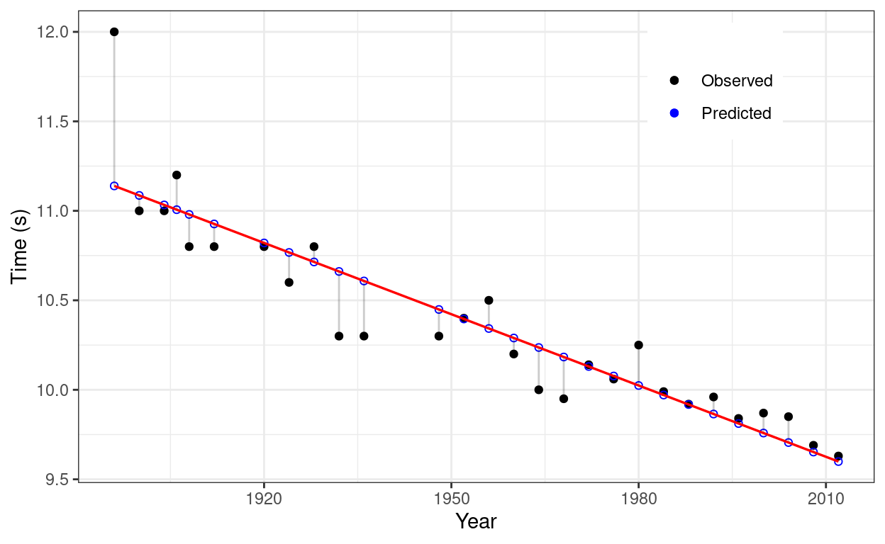
Figure 1: Limitation of deterministic linear model: unable to model the fluctuation.
\[\begin{equation}
t_{n} = \pmb{\omega}^{T}\pmb{x_{n}} + \epsilon_{n}, \;
\epsilon_{n} \sim \mathcal{N}(0, \sigma^2)
\label{eq:eq1}
\end{equation}\]
where \[ \pmb{\omega}=\begin{bmatrix} \omega_{0} \\ \omega_{1} \\ \vdots \\ \omega_{K} \end{bmatrix} \qquad \pmb{x}=\begin{bmatrix} 1 \\ x \\ x^2 \\ \vdots \\ x^{K} \end{bmatrix}. \]
Since \(\epsilon_{n}\) is a random variable with norm distribution, so is \(t_{n}\). The best model means we want to find the best values for \(\pmb{\omega}\) to maximize the following joint conditional density (\ref{eq:eq2}). This approach is called the maximum likelihood approach.
\[\begin{equation} \begin{split} \mathcal{L} & = p(t_1, \dots, t_N \mid x_1, \dots, x_N, \pmb{\omega}, \sigma^2) \\ & = \prod_{n=1}^{N}p(t_n \mid x_n, \pmb{\omega}, \sigma^2) \\ & = \prod_{n=1}^{N}\mathcal{N}(\pmb{\omega}^{T}\pmb{x_{n}}, \sigma^2) \\ & = \prod_{n=1}^{N}\frac{1}{\sqrt{2\pi\sigma^2}}\exp\{-\frac{1}{2\sigma^2} (t_n - \pmb{\omega}^{T}\pmb{x_n})^2\} \end{split} \label{eq:eq2} \end{equation}\]
Analytical solution
It is easier to deal with the natural logarithm of the likelihood function (\ref{eq:eq2})
\[\begin{equation} \begin{split} log\; \mathcal{L} & = \sum_{n=1}^{N}log(\frac{1}{\sqrt{2\pi\sigma^2}}\exp\{-\frac{1}{2\sigma^2} (t_n - \pmb{\omega}^{T}\pmb{x_n})^2\}) \\ & = -\frac{N}{2} log 2\pi - N log \sigma - \frac{1}{2 \sigma^2}\sum_{n=1}^{N}(t_n - \pmb{\omega}^{T}\pmb{x_n})^2 \end{split} \label{eq:eq3} \end{equation}\]
As for the least squares solutions derived in Chapter1, we can find the optimal solutions by taking derivatives and setting them to zero.
\[\begin{equation} \frac{\partial log\mathcal{L}}{\partial \pmb{\omega}} = \frac{1}{\sigma^2}(\pmb{X}^{T}\pmb{t} - \pmb{X}^{T}\pmb{X}\pmb{\omega}) = 0 \label{eq:eq4} \end{equation}\]
or \[\begin{equation} \pmb{X}^{T}\pmb{X}\pmb{\omega} = \pmb{X}^{T}\pmb{t} \label{eq:eq5} \end{equation}\]
\[ \pmb{t}=\begin{bmatrix} t_{1} \\ t_{2} \\ \vdots \\ t_{N} \end{bmatrix} \qquad \pmb{X}=\begin{bmatrix} \pmb{x_{1}}^{T} \\ \pmb{x_{2}}^{T} \\ \vdots \\ \pmb{x_{N}}^{T} \end{bmatrix} =\begin{bmatrix} 1 & x_{1} & x_{1}^2 & \dots & x_{1}^K \\ 1 & x_{2} & x_{2}^2 & \dots & x_{2}^K \\ \vdots & \vdots & \vdots & \ddots & \vdots \\ 1 & x_{N} & x_{N}^2 & \dots & x_{N}^K \end{bmatrix} \]
Similarly,
\[\begin{equation} \frac{\partial log \mathcal{L}}{\sigma} = -\frac{N}{\sigma} + \frac{1}{\sigma^3}\sum_{n=1}^{N}(t_n - \pmb{\omega}^{T}\pmb{x_n})^2 = 0 \label{eq:eq6} \end{equation}\]
or \[\begin{equation} \sigma^2 = \frac{1}{N}\sum_{n=1}^{N}(t_n - \pmb{\omega}^{T}\pmb{x_n})^2 \label{eq:eq7} \end{equation}\]
So we have derived the estimates of \(\pmb{\omega}\) and \(\sigma^2\)
\[\begin{equation} \widehat{\pmb{\omega}} = (\pmb{X}^{T}\pmb{X})^{-1}\pmb{X}^{T}\pmb{t} \label{eq:eq8} \end{equation}\]
\[\begin{equation} \widehat{\sigma^2} = \frac{1}{N}(\pmb{t}^{T}\pmb{t} - \pmb{t}^{T}\pmb{X}\widehat{\pmb{\omega}}) \label{eq:eq9} \end{equation}\]
Since \(\pmb{t}\) is a random variable, so are the estimates \(\widehat{\pmb{\omega}}\) and \(\widehat{\sigma^2}\). How are they related to the true value \(\pmb{\omega}\) and \(\sigma^2\)?
2.2 Uncertainty in estimates of parameters
Since \[\begin{equation} p(\pmb{t} \mid \pmb{X}, \pmb{\omega}, \sigma^2) = \mathcal{N}(\pmb{X}\pmb{\omega}, \sigma^2\pmb{I}), \label{eq:eq10} \end{equation}\]
\[\begin{equation} \begin{split} \pmb{E}_{p(\pmb{t} \mid \pmb{X}, \pmb{\omega}, \sigma^2)} \{\hat{\pmb{\omega}}\} & = \int \hat{\pmb{\omega}} p(\pmb{t} \mid \pmb{X}, \pmb{\omega}, \sigma^2) d\pmb{t} \\ & = (\pmb{X}^{T}\pmb{X})^{-1}\pmb{X}^{T} \int \pmb{t} p(\pmb{t} \mid \pmb{X}, \pmb{\omega}, \sigma^2) d\pmb{t} \\ & = (\pmb{X}^{T}\pmb{X})^{-1}\pmb{X}^{T}\pmb{X}\pmb{\omega} \\ & = \pmb{\omega} \end{split} \label{eq:eq11} \end{equation}\]
Equation (\ref{eq:eq11}) tells us that the expected value of our estiamtes \(\hat{\pmb{\omega}}\) is the true parameter value. But in practice, we usually obtain a point estimate. We should ask how far the point estimate is from the true value. This question is answered by calculating the covaiance matrix. The diagonal elements tell us how much variability we might expect for an individual estimate. The off-diagonal elements tell us how the parameters are related. If the values are high and positive, increasing one will require increasing the other to maintain a good model. If the values are high and negative, increasing one will require decreasing the other to maintain a good model. If the values are close to zero, the parameters are independent. Let us calculate the covariance matrix.
Equation (\ref{eq:eq10}) tells us \[ cov\{\pmb{t}\} = \sigma^2\pmb{I} = \pmb{E}_{p(\pmb{t} \mid \pmb{X}, \pmb{\omega}, \sigma^2)}\{\pmb{t}\pmb{t}^T\} - \pmb{E}_{p(\pmb{t} \mid \pmb{X}, \pmb{\omega}, \sigma^2)}\{\pmb{t}\}\pmb{E}_{p(\pmb{t} \mid \pmb{X}, \pmb{\omega}, \sigma^2)}\{\pmb{t}^T\} \] Rearranging this expression to obtain \[ \pmb{E}_{p(\pmb{t} \mid \pmb{X}, \pmb{\omega}, \sigma^2)}\{\pmb{t}\pmb{t}^T\} = \sigma^2\pmb{I} + \pmb{E}_{p(\pmb{t} \mid \pmb{X}, \pmb{\omega}, \sigma^2)}\{\pmb{t}\}\pmb{E}_{p(\pmb{t} \mid \pmb{X}, \pmb{\omega}, \sigma^2)}\{\pmb{t}^T\} = \sigma^2\pmb{I} + \pmb{X}\pmb{\omega} (\pmb{X}\pmb{\omega})^T \]
Therefore,
\[\begin{equation} \begin{split} \pmb{E}_{p(\pmb{t} \mid \pmb{X}, \pmb{\omega}, \sigma^2)} \{ \hat{\pmb{\omega}}\hat{\pmb{\omega}}^T\} & = \pmb{E}_{p(\pmb{t} \mid \pmb{X}, \pmb{\omega}, \sigma^2)} \{\left((\pmb{X}^{T}\pmb{X})^{-1}\pmb{X}^{T}\pmb{t}\right)\left((\pmb{X}^{T}\pmb{X})^{-1}\pmb{X}^{T}\pmb{t}\right)^T\}\\ & = (\pmb{X}^{T}\pmb{X})^{-1}\pmb{X}^{T}\pmb{t}\pmb{t}^T\pmb{X}(\pmb{X}^{T}\pmb{X})^{-1}\\ & = \pmb{\omega}\pmb{\omega}^T + \sigma^2(\pmb{X}^{T}\pmb{X})^{-1} \end{split} \label{eq:eq12} \end{equation}\]
Thus, \[\begin{equation} \begin{split} cov\{\hat{\pmb{\omega}}\} & = \pmb{E}_{p(\pmb{t} \mid \pmb{X}, \pmb{\omega}, \sigma^2)} \{ \hat{\pmb{\omega}}\hat{\pmb{\omega}}^T\} - \pmb{E}_{p(\pmb{t} \mid \pmb{X}, \pmb{\omega}, \sigma^2)} \{\hat{\pmb{\omega}}\}\pmb{E}_{p(\pmb{t} \mid \pmb{X}, \pmb{\omega}, \sigma^2)} \{\hat{\pmb{\omega}}^T\}\\ & = \sigma^2(\pmb{X}^{T}\pmb{X})^{-1} \end{split} \label{eq:eq13} \end{equation}\]
So we know the expected value of \(\hat{\pmb{\omega}}\) is the true value, and how to estimate the uncertainty of individual estimate. We would ask the same questions regarding the estimate \(\widehat{\sigma^2}\).
First, if \(\pmb{t} \sim \mathcal{N}(\pmb{\mu}, \pmb{\Sigma})\), we can derive that
\[ \pmb{E}_{p(\pmb{t})} \{\pmb{t}^T\pmb{A}\pmb{t}\} = \pmb{\mu}^T \pmb{A} \pmb{\mu} + Tr(\pmb{A}\pmb{\Sigma}) \]
where \(Tr()\) is the trace function, i.e. the sum of the diagonal elements of a square matrix.
From equations (\ref{eq:eq8}) and (\ref{eq:eq9}), we obtain
\[\begin{equation} \begin{split} \pmb{E}_{p(\pmb{t} \mid \pmb{X}, \pmb{\omega}, \sigma^2)} \{ \widehat{\sigma^2} \} & = \frac{1}{N} \pmb{E}_{p(\pmb{t} \mid \pmb{X}, \pmb{\omega}, \sigma^2)} \{\pmb{t}^{T}\pmb{t} - \pmb{t}^{T}\pmb{X}\hat{\pmb{\omega}}\}\\ & = \frac{1}{N} \pmb{E}_{p(\pmb{t} \mid \pmb{X}, \pmb{\omega}, \sigma^2)} \{\pmb{t}^{T}\pmb{t}\} - \frac{1}{N} \pmb{E}_{p(\pmb{t} \mid \pmb{X}, \pmb{\omega}, \sigma^2)}\{\pmb{t}^{T}\pmb{X}(\pmb{X}^{T}\pmb{X})^{-1}\pmb{X}^{T}\pmb{t}\}\\ & = \sigma^2 (1 - \frac{D}{N}) \end{split} \label{eq:eq14} \end{equation}\]
where \(D\) is the number of columns in \(\pmb{X}\) (the number of parameters/attributes), and \(N\) is the number of rows in \(\pmb{X}\) (the number of data points). So the estimator is biased. But we can increase \(N\) so that the expected value of estimates converges to the true value.
2.3 Uncertainty in prediction
Since \(\pmb{\hat{\omega}}\) is a random variable, so is the prediction \(t_{new} = \hat{\pmb{\omega}}^T x_{new}\). However, from equation (\ref{eq:eq11}), we obtain \[ \pmb{E}_{p(\pmb{t} \mid \pmb{X}, \pmb{\omega}, \sigma^2)} \{t_{new}\} = \pmb{\omega}^T x_{new} \] This tells us that the expected value of our predictions is the true value. We ask how reliable a point prediction is. To answer this question, we need to calculate the variance. Similar to the derivation of equation (\ref{eq:eq13}), we can obtain
\[\begin{equation} \begin{split} \sigma_{new}^2 & = \pmb{E}_{p(\pmb{t} \mid \pmb{X}, \pmb{\omega}, \sigma^2)}\{t_{new}^2\} - \left(\pmb{E}_{p(\pmb{t} \mid \pmb{X}, \pmb{\omega}, \sigma^2)}\{t_{new}\}\right)^2 \\ & = \sigma^2 x_{new}^{T}(\pmb{X}^{T}\pmb{X})^{-1}x_{new} \end{split} \label{eq:eq15} \end{equation}\]
This implies that the uncertainty of prediction is proportional to the uncertainty of the estimate of parameters. If we are less sure on the parameter estimates, we are going to be less sure of the predictions too.
2.4 Numerical solution
We first generate a set of synthetic data using
\[\begin{equation} t = 5 x^3 - x^2 + x + \epsilon, \; \epsilon \sim \mathcal{N}(0, 300) \label{eq:eq16} \end{equation}\]
## Sample data from the true function
# $y = 5x^3-x^2+x$
N = 100 # Number of training points
y <- runif(N)
x = sort(10*y-5)
t = 5*(x^3) - (x^2) + x
noise_var = 300
t = t + rnorm(length(x))*sqrt(noise_var)
plot(x, t)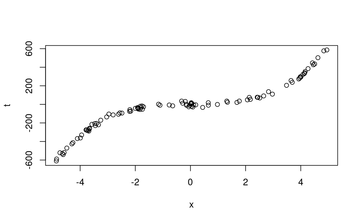
Figure 2: Synthetic data generated from equation (16).
Let us remove part of the data to see whether we are able to predict them.
# Chop out some x data
pos = which(x>0 & x<2)
x = x[-pos]
t = t[-pos]
plot(x,t)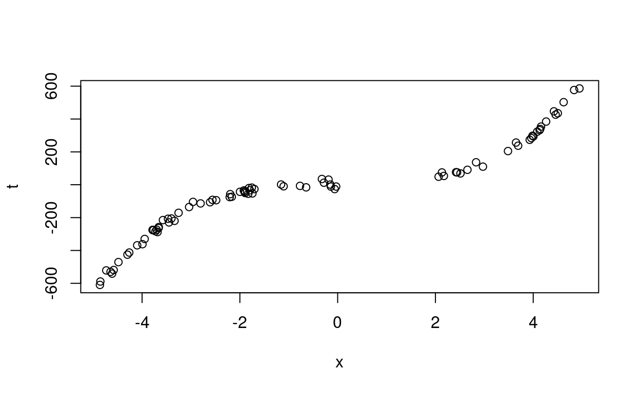
Figure 3: Data between 0 and 2 are removed.
We test different models from first to eighth order.
## Fit models of various orders
orders = c(1:8)
testx = seq(-5,5,0.1)
for(i in 1:length(orders)){
  X = matrix(x^0)
  testX = matrix(testx^0)
  for(k in 1:orders[i]){
    X = cbind(X,x^k)
    testX = cbind(testX,testx^k)
  }
  w = solve(t(X)%*%X)%*%t(X)%*%t
  ss = (1/N)*(t(t)%*%t - t(t)%*%X%*%w)
  testmean = testX%*%w
  testvar = c(ss)*diag(testX%*%solve(t(X)%*%X)%*%t(testX))
  # Plot the data and predictions
  plot(x,t,main=paste('Order',orders[i]),col="red",pch=16)
  errbar(testx,testmean, testmean+testvar, testmean-testvar,add=TRUE,cex=0.5)
}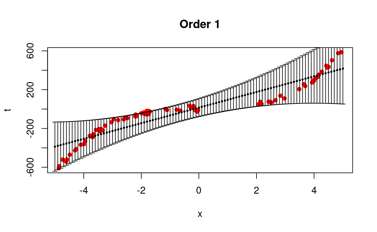
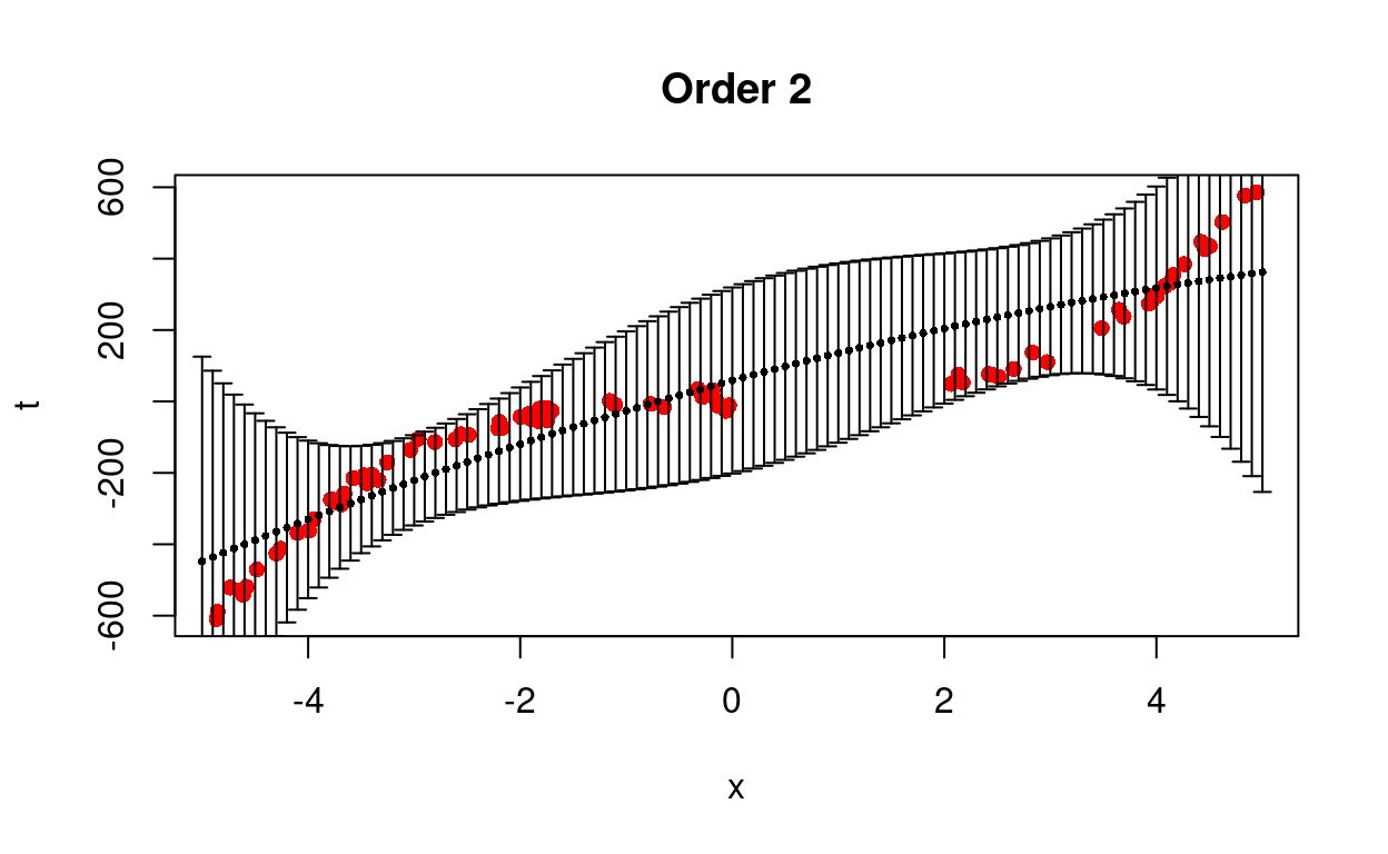
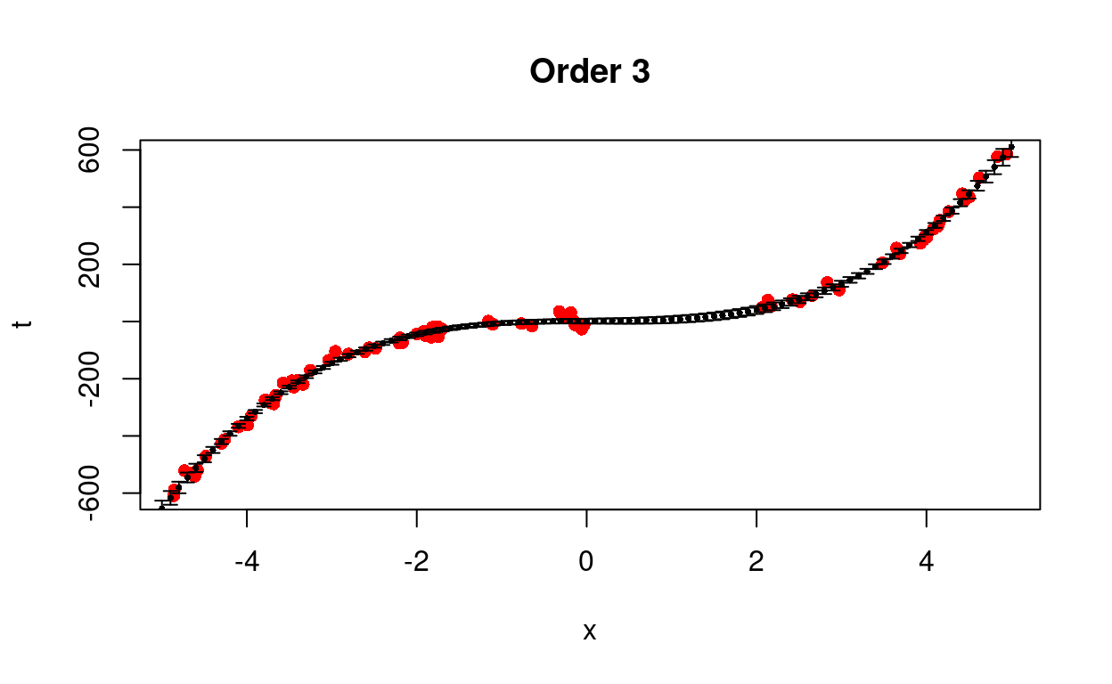

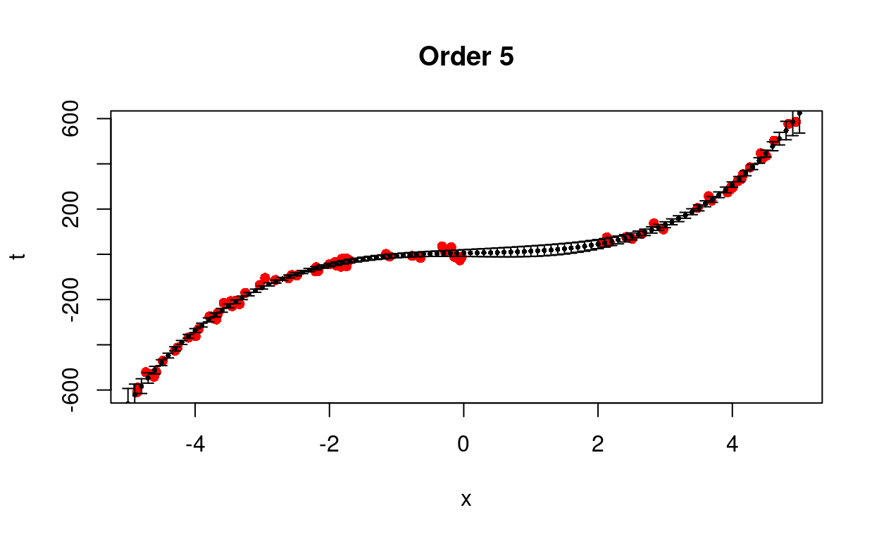

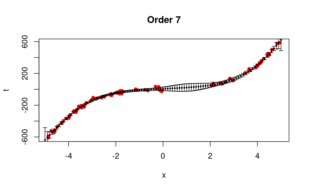
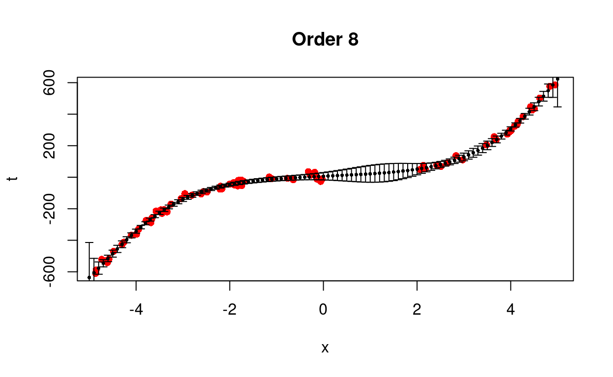
Figure 4: Predict removed data using different models.
We see that the cubic model is better able to predict the trend with less uncertainty.
2.5 Discussion
The advantage of the maximum likelihood method is that it is able to give the uncertainty of an estimate:
\[ \pmb{E}_{p(\pmb{t} \mid \pmb{X}, \pmb{\omega}, \sigma^2)} \{\hat{\pmb{\omega}}\} = \pmb{\omega} \]
\[ cov\{\hat{\pmb{\omega}}\} = \sigma^2(\pmb{X}^{T}\pmb{X})^{-1} \]
We know that the parameter \(\pmb{\omega}\) optimizes the likelihood function (\ref{eq:eq2}), it can be shown
\[\begin{equation} cov\{\hat{\pmb{\omega}}\} = \sigma^2(\pmb{X}^{T}\pmb{X})^{-1} = - \left(\frac{\partial^2 log\mathcal{L}}{\partial \pmb{\omega}\partial \pmb{\omega}^T} \right)^{-1} \label{eq:eq17} \end{equation}\]
This results tells us that the uncertainty in the parameter estimate as described by the covariance matrix is directly related to the second derivative of the log-likelihood. The second derivative of the log-likelihood tells us about the curvature of the likelihood function. Suppose the true model is \(t = 3x - 2\). We add some Gaussian noise. In one case \(\sigma = 0.5\). In the second case \(\sigma = 0.2\). Figure 5 shows two generated systhetic datasets.
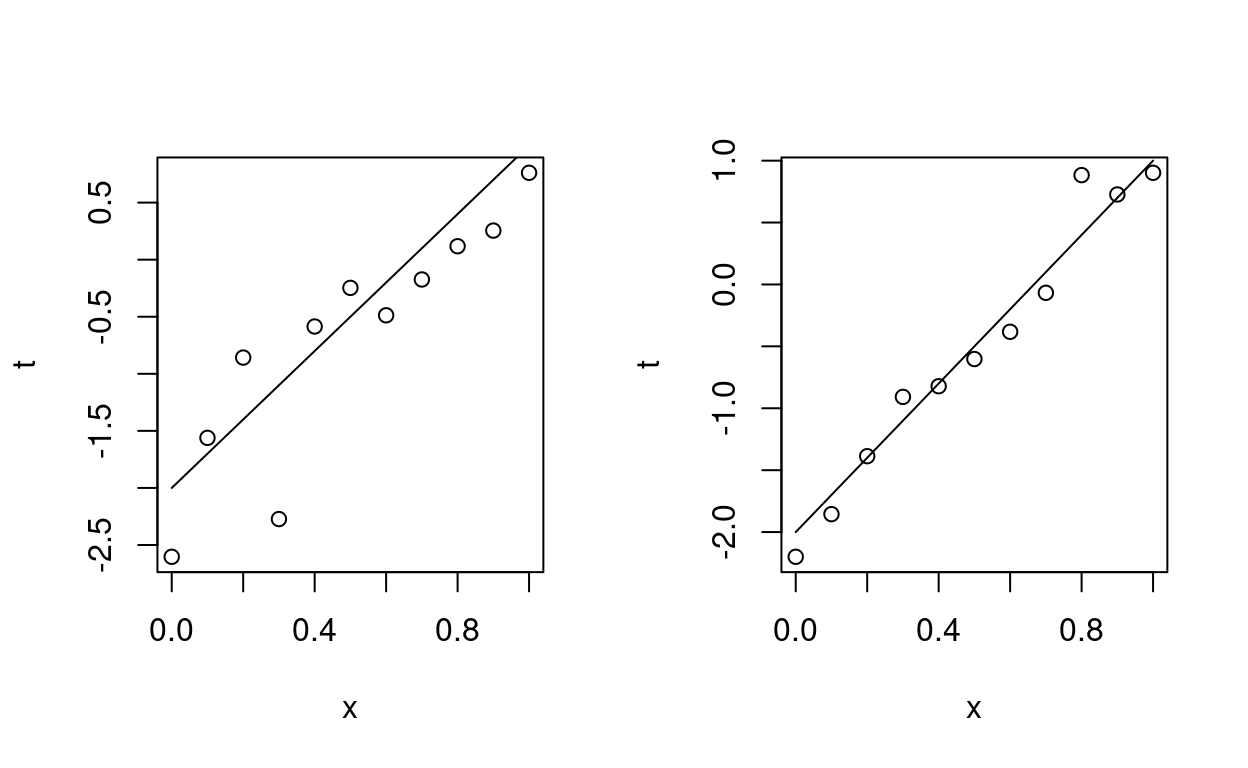
Figure 5: Two sets of synthetic data with different noise level.
The following contour plots shows the corresponding likelihood functions as a function of \(\hat{\pmb{w}}\).
##
## Attaching package: 'pracma'
## The following object is masked from 'package:Hmisc':
##
## ceil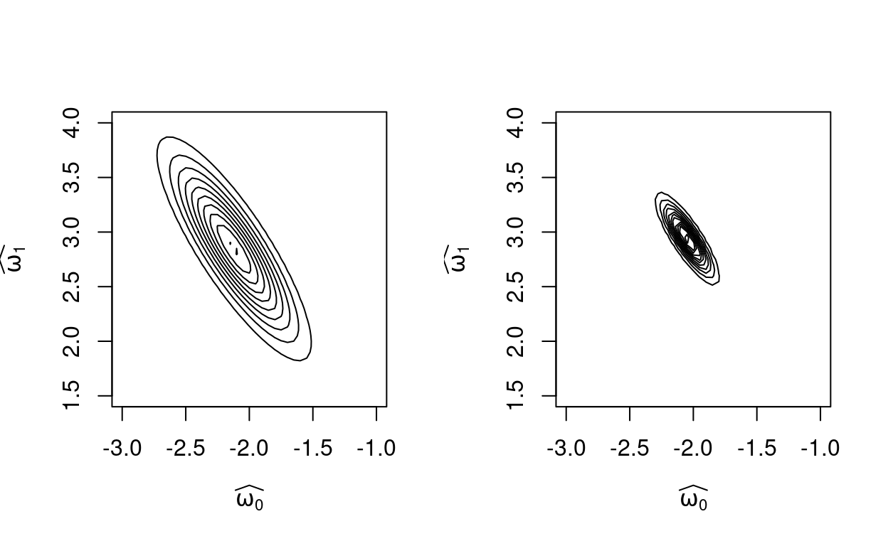
Figure 6: The curvature of likilihood functions dependeing data noise.