Click Start Over menu at the left bottom to start Back to Contents
1. The Problem
Here is a general description of a dynamic system
\[ \begin{equation} \dot{\pmb{x}} = f(\pmb{x}, t, \mu; \beta) \end{equation} \label{dynamics} \]
where \(\pmb{x}\) is a state vector varying with time \(t\); \(\mu\) is the control parameters; \(\beta\) is the physical parameters; \(f\) is the dynamics function (vector field); In the case that \(f\) is unknown or \(f\) is too complicated to solve Eq. (\ref{dynamics}), but we do have measured data about \(\pmb{x}\), can we approximate Eq.(\ref{dynamics}) by a linear differential systems using the measured data? That is to say whether we can find a matrix \(\pmb{A}\) such that the solution \(\pmb{\tilde{x}}\) to
\[ \begin{equation} \dot{\pmb{\tilde{x}}} = \pmb{A}\pmb{\tilde{x}} \end{equation} \label{linear} \]
is a good approximation to the solution to Eq. (\ref{dynamics}) in a least-square sense: \(\|\pmb{\tilde{x}} - \pmb{x}\| \ll 1\).
Example 1. Nonlinear dynamics system converted into linear systems.
Consider the following non-linear system:
\[ \begin{equation} \begin{cases} \dot{x}_1 = \mu x_1 \\ \dot{x}_2 = \lambda (x_2 - x_{1}^2) \end{cases} \end{equation} \label{example1org} \]
Let \(y_1 = x_1, y_2 = x_2, y_3 = x_{1}^2\). Then Eqs. (\ref{example1org}) are transformed into a linear system:
\[ \frac{d}{dt}\left[\begin{array}{c} y_1\\ y_2 \\ y_3 \end{array} \right]= \left[\begin{array}{ccc} \mu & 0 & 0\\ 0 & \lambda & -\lambda\\ 0 & 0 & 2\mu \end{array} \right] \left[\begin{array}{c} y_1\\ y_2 \\ y_3 \end{array} \right] \]
Example 2. Nonlinear dynamics system converted into linear systems.
Consider the following non-linear system
\[ \begin{equation} \frac{d}{dt}x=x^2 \end{equation} \label{example2} \]
If we set \(y_1 = x, y_2 = x^2\), Eqs. (\ref{example2}) are converted into another non-linear system:
\[ \frac{dy_1}{dt} = y_2 \\ \frac{dy_2}{dt} = 2x\dot{x} = 2x^3=2y_1y_2 \]
However, if we set \(y = e^{-1/x}\), Eqs. (\ref{example2}) are converted into a linear system:
\[ \frac{dy}{dt}=y\times x^{-2} \frac{dx}{dt}=y \]
2. Exact Dynamic Mode Decomposition
Let \(\pmb{x}_1, \pmb{x}_2, \cdots, \pmb{x}_{m}\) be a sequence of snapshots/measurements of the system states over \(m\) evenly spaced time periods. It is discovered that the linear system (\ref{linear}) using \(\pmb{A}\) such that \(\pmb{x}_{k+1} = \pmb{A}\pmb{x}_{k}\), \(k=1, 2, \cdots, m-1\), is a good approximation to the general dynamic system (\ref{dynamics}). Such an \(\pmb{A}\) is called the Koopman operator.
Let \(\pmb{X}=[\pmb{x}_1, \pmb{x}_2, \cdots, \pmb{x}_{m-1}]\), \(\pmb{X'}=[\pmb{x}_2, \pmb{x}_3, \cdots, \pmb{x}_{m}]\). Since
\[ \begin{equation} \pmb{X'}=\pmb{A}\pmb{X} \end{equation} \label{exactDMD} \]
the matrix \(\pmb{A}\) can formally computed from the data as
\[ \pmb{A} = \pmb{X'}\pmb{X}^{\dagger} \]
where \(\pmb{X}^{\dagger}\) denotes the pseudo inverse of \(\pmb{X}\).
For huge data, it is difficult to explicitly compute and store \(\pmb{A}\), and then solve Eq.(\ref{linear}). The goal of dynamic mode decomposition (DMD) is to find an approximate solution to Eq.(\ref{linear}) associated with \(\pmb{A}\) without explicitly computing it.
3. DMD algorithm
1 Do singular value decomposition (svd) of \(\pmb{X}\):
\[ \pmb{X} = \pmb{U}\pmb{\Sigma}\pmb{V}^{*}. \]
\[ \pmb{X'} = \pmb{A}\pmb{X} = \pmb{A}\pmb{U}\pmb{\Sigma}\pmb{V}^{*}. \]
\[ \pmb{A} = \pmb{X'} \pmb{V} \pmb{\Sigma}^{-1} \pmb{U}^{*}. \]
Then based on the variance captured by the singular values and the application of the algorithm, the number of desired reconstruction rank can be chosen.
2 Using the chosen rank, construct a low-dimensional matrix \(\pmb{\tilde{A}}\) having the same eigenvalues as \(\pmb{A}\):
\[ \pmb{\tilde{A}} = \pmb{U}^{*}\pmb{A}\pmb{U} = \pmb{U}^{*}\pmb{X'}\pmb{V}\pmb{\Sigma}^{-1} \]
3 Solve the low-dimensional eigenvalue problem:
\[ \pmb{\tilde{A}}\pmb{W}=\pmb{W}\pmb{\Lambda} \]
Since
\[ \pmb{\tilde{A}}\pmb{W} = \pmb{U}^{*}\pmb{A}\pmb{U}\pmb{W}=\pmb{W}\pmb{\Lambda}, \]
\[ \pmb{A}\pmb{U}\pmb{W}=\pmb{U}\pmb{W}\pmb{\Lambda}. \]
Thus \(\pmb{\Phi}\equiv \pmb{U}\pmb{W}\) is the eigenvectors (DMD modes) of \(\pmb{A}\) associated with eigenvalues \(\pmb{\Lambda}\). The solution to (\ref{linear}) can be approximated by
\[ \begin{equation} \hat{\pmb{x}}_k = \pmb{A}^{k-1}\pmb{x}_1 =\pmb{\Phi}\pmb{\Lambda}^{k-1}\pmb{b} \end{equation} \label{linearsol} \]
where \(\pmb{b}=\pmb{\Phi}^{\dagger}\pmb{x}_1\). This is also the approximate solution to Eq. (\ref{dynamics}). This is different from eigenvector expansion using Taylor expansion which only makes sense of square matrix.
We can change the units from snapshots \(k\) (observed at every \(\Delta t\)) to time \(t\), then Eq. (\ref{linearsol}) becomes
\[ \begin{equation} \hat{\pmb{x}}(t) =\pmb{\Phi}\exp({\pmb{\Omega} t})\pmb{b} \end{equation} \label{linearsolt} \]
where \(\pmb{\Omega} \equiv log(\pmb{\Lambda})/\Delta t\).
4. Numerical Examples
Here is the basic DMD algorithm implemented in R:
basicDMD <- function(data, rank) {
  r <- rank
  m <- dim(data)[2]
  X1 <- data[, 1:(m-1)]
  X2 <- data[, 2:m]
  X1.svd <- svd(X1)
  Ur <- X1.svd$u[, 1:r]
  Sr <- diag(1/X1.svd$d[1:r])   # r > 1
  Vr <- X1.svd$v[, 1:r]
  Ar <- t(Ur) %*% X2 %*% Vr %*% Sr
  Ar.eig <- eigen(Ar)
  dmdModes <- Ur %*% Ar.eig$vectors
  dmdEigs <- Ar.eig$values
  return(list(dmdModes=dmdModes, dmdEigs=dmdEigs))
}
Example 3. Suppose the first five columns of X are collected data. Predict the sixth column.
Step 1. Prepare data and choose rank
# svd
X <- matrix(c(-2, 6, 1, 1, -1, -1, 5, 1, 2, -1, 0, 4, 2,  1, -1, 1, 3, 2, 2, -1, 2, 2, 3, 1, -1, 3, 1, 3, 2, -1), nrow = 5)
X1 <- X[, 1:4]
X1.svd <- svd(X1)
X1.svd$d
## [1] 1.036826e+01 2.743190e+00 9.869640e-01 4.904416e-16plot(seq_along(X1.svd$d), X1.svd$d/sum(X1.svd$d), xlab="Index", ylab="Percent")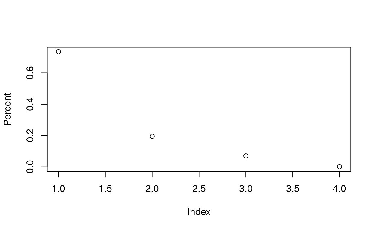
Step 2. Perform DMD
dmd <- basicDMD(X[,1:5], 2)Step 3. Reconstruct solution and make prediction
library(MASS)  # pseudo inverse
Psi <- dmd$dmdModes
Psi.ginv <- ginv(Psi)
b <- Psi.ginv %*% X[,1]
omega <- dmd$dmdEigs
xDMD <- sapply(0:6, function(x) Psi %*% diag(omega^x) %*% b)
xDMD
## [,1] [,2] [,3] [,4] [,5]
## [1,] -2.0124798+0i -0.9926017+0i 0.0157601+0i 0.9943308+0i 1.9259200+0i
## [2,] 5.9801634+0i 5.0326802+0i 4.0200256+0i 2.9627972-0i 1.8818128+0i
## [3,] 0.8877005+0i 1.3190756+0i 1.7134837+0i 2.0647265+0i 2.3675838+0i
## [4,] 1.1717237+0i 1.4193452+0i 1.6335249+0i 1.8112878+0i 1.9504184+0i
## [5,] -0.9919209-0i -1.0100196-0i -1.0089464-0i -0.9892820-0i -0.9519332-0i
## [,6] [,7]
## [1,] 2.7947073+0i 3.5864945+0i
## [2,] 0.7977198-0i -0.2693813-0i
## [3,] 2.6178813+0i 2.8125365+0i
## [4,] 2.0494787+0i 2.1078128+0i
## [5,] -0.8981068-0i -0.8292783-0iExample 4. Reconstruct Solution
Suppose the solution to a nonlinear system is
\[ x(t; \xi)=sech(\xi + 3)\exp(i2.3t) + 2 sech(\xi)tanh(\xi)\exp(i2.8t) \]
Let us reconstruct the solution using DMD.
Step 1. Generate data
library(pracma)
f <- function(xi, t) {
  sech(xi + 3) * exp(2.3i * t) + 2 * sech(xi)* tanh(xi) * exp(2.8i * t)
}
xi <- seq(-5, 5, length.out = 128)
t <- seq(0, 4 * pi, length.out = 256)
xitgrid <- meshgrid(xi, t)
X <- f(xitgrid$X, xitgrid$Y)
Step 2. Choose rank
# change x columnwise to t columnwise
Xt <- t(X)
m <- dim(Xt)[2]
X1 <- Xt[, 1:(m-1)]
X2 <- Xt[, 2:m]
X1.svd <- svd(X1)
plot(seq_along(X1.svd$d), X1.svd$d/sum(X1.svd$d))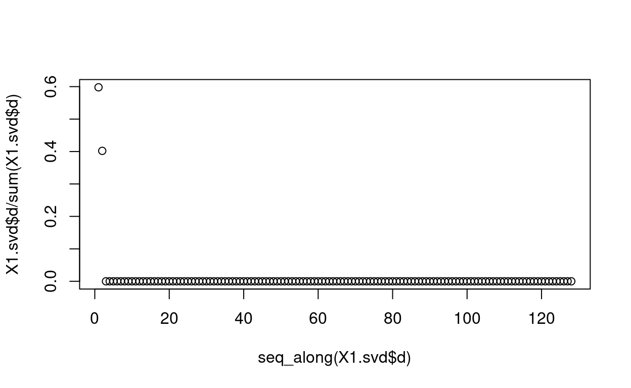
Step 3. Compute DMD mode
dmd <- basicDMD(Xt, 2)
#dmd$dmdModes
#dmd$dmdEigs
# plot modes
mode.Re <- Re(dmd$dmdModes)
plot(xi, mode.Re[,1], type="l", ylim=c(min(mode.Re), max(mode.Re)), xlab="", ylab="")
lines(xi, mode.Re[,2], col="red")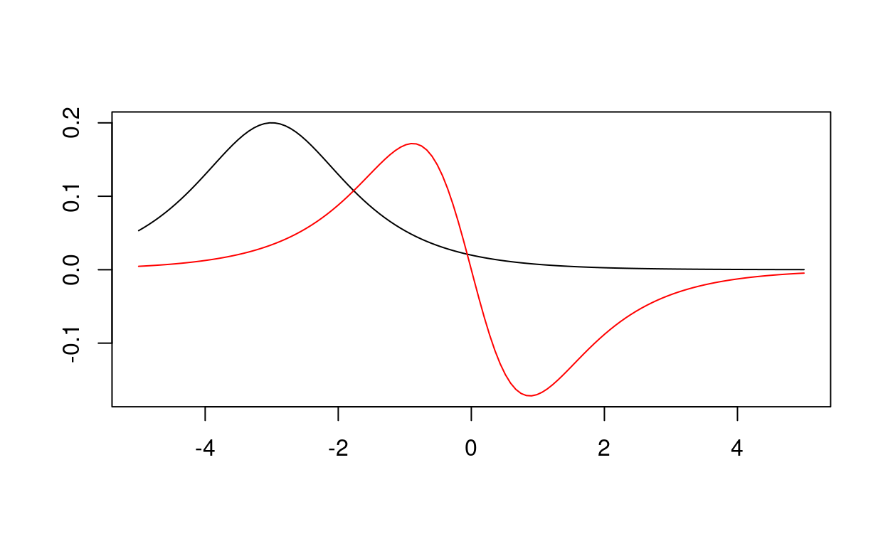
Step 3. Reconstruct solution and make prediction
library(MASS)  # pseudo inverse
Psi <- dmd$dmdModes
Psi.ginv <- ginv(Psi)
b <- Psi.ginv %*% Xt[,1]
omega <- dmd$dmdEigs
xDMD <- sapply(0:length(t), function(x) Psi %*% diag(omega^x) %*% b)library(plot3D)## Warning: no DISPLAY variable so Tk is not availablepar(mfrow=c(1, 2))
surf3D(xitgrid$X, xitgrid$Y, Re(X))
surf3D(xitgrid$X, xitgrid$Y, t(Re(xDMD[,-dim(xDMD)[2]])))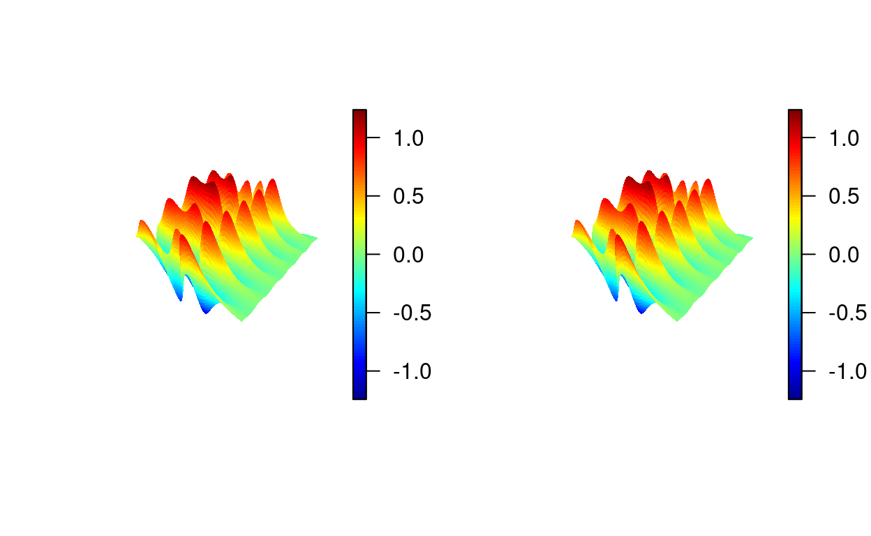
References
Brunton et al., Extractingspatial–temporalcoherentpatternsinlarge-scaleneuralrecordingsusingdynamicmodedecomposition. Journal of Neuroscience Methods. 2016.