Basic understanding of the algorithm

Let \(X\) be a column centered data matrix of \(n \times d\) size. Each row is a data point with \(d\) features. Then the \(d \times d\) covariance matrix of \(X\) is given by \(C = X^T X / (n-1)\). Its eigenvectors are principal axes (PAs) of \(X\) and eigenvalues are PC variances of \(X\). The components of \(X\) on the principal axes are called principal components.

Let \(X=U_{n\times r}D_{r\times r}V_{d\times r}^T\) be the SVD decomposition of \(X\), where \(r\le d\) is the rank of \(X\). Then \(C = VDU^TUDV^T/(n-1) = VD^2V^T/(n-1)\). Therefore \(V\) are eigenvectors of \(C\) (PAs of \(X\)), and The diagonal entries of \(D^2/(n-1)\) are non-zero eigenvalues of \(C\) (PC variances of \(X\)). Consider the transformation

\[\begin{equation} Z = X V \sqrt{\frac{n-1}{D^2}}\frac{1}{\sqrt{n-1}}=X V \Lambda^{-1/2}\frac{1}{\sqrt{n-1}} \label{eq:standardproj} \end{equation}\]

where \(\Lambda\) is the diagonal matrix whose diagonal entries are the non-zero eigenvalues of \(C\).

Since

\[ \begin{align} Z^T Z &= \sqrt{\frac{1}{D^2}} V^T X^T X V \sqrt{\frac{1}{D^2}} \\ &= \sqrt{\frac{1}{D^2}} V^T V D U^T U D V^T V \sqrt{\frac{1}{D^2}} = I, \end{align} \] \(Z\) is normalized. \(Z\) is the normalized principal components in the principal axes \(V\).

Remark 1. Since

\[ \begin{align} XX^T Z &= XX^T X V \Lambda^{-1/2}\frac{1}{\sqrt{n-1}} \\ &= X VD^2V^T V \Lambda^{-1/2}\frac{1}{\sqrt{n-1}} \\ & = (XV\Lambda^{-1/2}\frac{1}{\sqrt{n-1}})D^2 = ZD^2, \end{align} \] \(Z\) are the eigenvectors of \(XX^T/(n-1)\). \(D^2 / (n-1)\) are the eigenvalues of \(XX^T/(n-1)\).

Numerical Implementation

1. Get data

For illustration, we use a toy data matrix \(X\).

X <- matrix(data = c(2.5, 0.5, 2.2, 1.9, 3.1, 2.3, 2.0, 1.0, 1.5, 1.1,
                     2.4, 0.7, 2.9, 2.2, 3.0, 2.7, 1.6, 1.1, 1.6, 0.9), ncol = 2)
plot(X[,1], X[,2],xlab=expression("x"[1]), ylab=expression("x"[2]))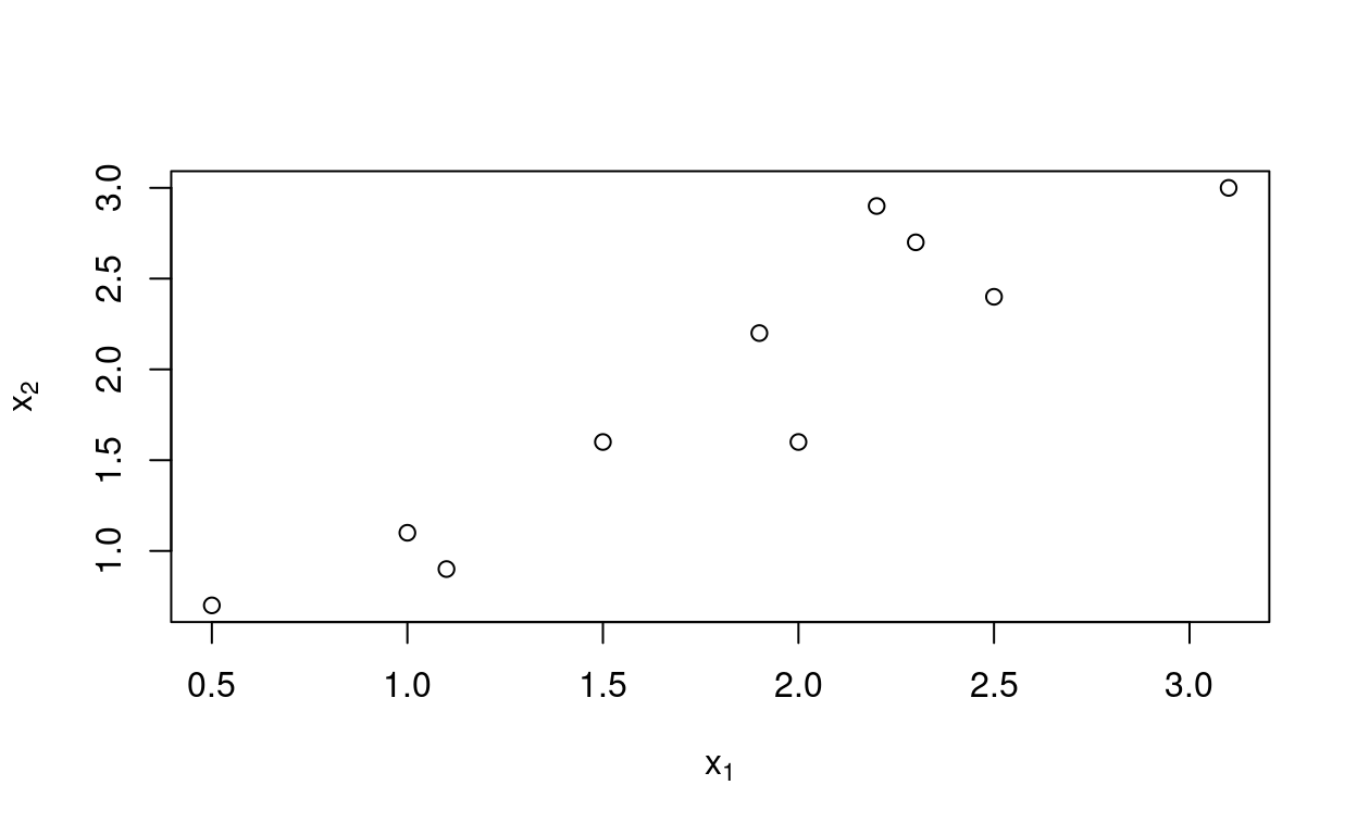

2. Convert \(X\) to a column-centered matrix

It is not necessary for calculating the covariance matrix, but it is necessary for performing projection.

# column mean-centering 
Xc <- apply(X, 2, function(y) y - mean(y))

3. Calculate the covariance matrix

C <- cov(Xc)

4. Get the eigenvalues and eigenvectors of the covariance matrix

C.eigen <- eigen(C)

5. Choose principal axes

The eigenvalues of \(C\) are used to find the proportion of the total variance explained by the components.

totalVar <- sum(C.eigen$values)
# one can check it equal to the total variance sum(diag(S)) 
totalVar == sum(diag(C))

## [1] TRUE

for (s in C.eigen$values) {
  print(s/totalVar)
}

## [1] 0.9631813
## [1] 0.03681869

The first eigenvalue account for \(96.3%\) of the total variance. So we choose the first eigenvector as the principal axis.

6. Project on the principal axis

# Set up figure layout
par(oma=c(0, 0, 0, 0), mar = c(4, 4.1, 2, 1), las="1", xpd=TRUE)
layout.matrix <- matrix(c(1, 2), nrow = 1, ncol = 2)
layout(mat = layout.matrix, heights = c(3.25), widths = c(3.25, 3.25))
# Plot principal component
plot(Xc, xlab=expression("x"[1]), ylab=expression("x"[2]))
x <- seq(-1.0, 1.0, 0.1)
lines(x, -x * C.eigen$vectors[1,2]/C.eigen$vectors[1,1], col='red')
# Principal components scaled to unit norm
r <- 2
V <- C.eigen$vectors[,1:r]
n <- dim(Xc)[1]
for (i in 1:r) {
V[,i] <- V[,i]/sqrt((n-1)*C.eigen$values[i])
}
PXc <- Xc %*% V
plot(PXc,  xlab="PC1", ylab="PC2")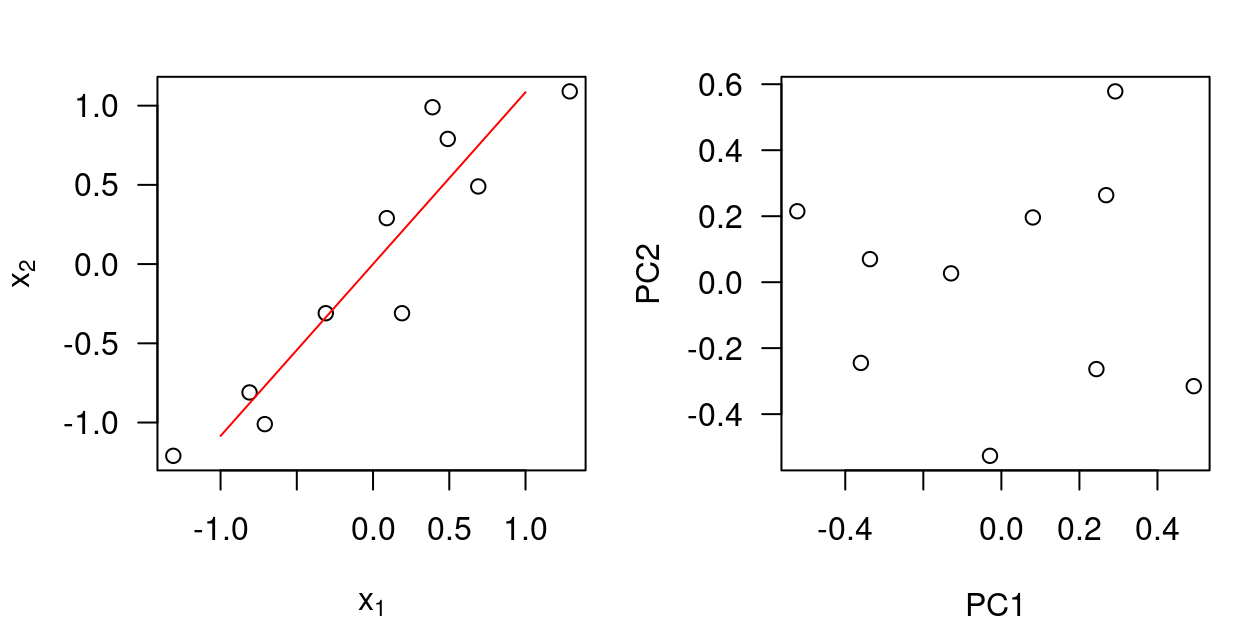

7. Verify Remark 1

gram <- Xc %*% t(Xc)/9
gram.eign <- eigen(gram)
round(gram.eign$values[1:2], 6) == round(C.eigen$values, 6)

## [1] TRUE TRUE

round(gram.eign$vectors[, 1], 6) == round(PXc[, 1], 6)

##  [1] TRUE TRUE TRUE TRUE TRUE TRUE TRUE TRUE TRUE TRUE

# difference in a scaling factor -1
round(gram.eign$vectors[, 2], 6) == round(-PXc[, 2], 6)

##  [1] TRUE TRUE TRUE TRUE TRUE TRUE TRUE TRUE TRUE TRUE

Validation

Compare with R function prcomp

pilots.pca <- prcomp(X)
pilots.pca

## Standard deviations (1, .., p=2):
## [1] 1.1331495 0.2215477
## 
## Rotation (n x k) = (2 x 2):
##             PC1        PC2
## [1,] -0.6778734  0.7351787
## [2,] -0.7351787 -0.6778734

Remark 2. The squares of the standard deviations equal to the eigenvalues of \(C\).

Remark 3. The PCs/Rotation are the same as the eigenvectors of \(C\) except for a scaling factor -1.

Basic understanding of the algorithm

Non-linear data (e.g. a curve in 2-D) may be linearized in a higher-dimensional space so that dimension of the data may be reduced. Kernel principal component analysis is to map the input space to a new higher-dimensional feature space. PCA is carried out in the new space.

Consider a feature map \(\phi: \mathbb{R}^2 \rightarrow \mathbb{R}^3\),

\[ \mathbf{x}= \begin{bmatrix} x_1 \\ x_2 \end{bmatrix} \mapsto \phi(\mathbf{x})=\begin{bmatrix} \phi_1 (\mathbf{x})\\ \phi_2 (\mathbf{x})\\ \phi_3 (\mathbf{x}) \end{bmatrix} \] The data matrix in \(\mathbb{R}^3\) is

\[ \Phi = \begin{bmatrix} \phi_1(\mathbf{x}_{1}) & \phi_2(\mathbf{x}_{1}) & \phi_3(\mathbf{x}_{1})\\ \phi_1(\mathbf{x}_{2}) & \phi_2(\mathbf{x}_{2}) & \phi_3(\mathbf{x}_{2})\\ \phi_1(\mathbf{x}_{3}) & \phi_2(\mathbf{x}_{3}) & \phi_3(\mathbf{x}_{3}) \\ \phi_1(\mathbf{x}_{4}) & \phi_2(\mathbf{x}_{4}) & \phi_3(\mathbf{x}_{4}) \end{bmatrix} = \begin{bmatrix} \phi(\mathbf{x}_{1})^T \\ \phi(\mathbf{x}_{2})^T \\ \phi(\mathbf{x}_{3})^T \\ \phi(\mathbf{x}_{4})^T \end{bmatrix} \]

In the feature space \(\mathbb{R}^3\), after centering the data, we can write the covariance matrix as

\[ \mathcal{C} = \frac{1}{n-1}\mathbf{\Phi}^T\mathbf{\Phi}=\frac{1}{n-1}\sum_{i=1}^n \phi(\mathbf{x}_i)\phi(\mathbf{x}_i)^T \] Remark 4. If \(\phi\) is a linear transformation:

\[ \begin{bmatrix} x_1 \\ x_2 \end{bmatrix} \mapsto \begin{bmatrix} x_1 \\ x_2 \end{bmatrix}, \]

then \(\mathcal{C}\) reduces to standard \(C\).

Consider the eigenvalue equation

\[\begin{equation} \mathcal{C} \mathbf{v} = \lambda \mathbf{v} \label{eq:feateigen} \end{equation}\]

i.e. 

\[ \frac{1}{n-1} \sum_{i=1}^n \phi(\mathbf{x}_i)(\phi(\mathbf{x}_i)^T\mathbf{v}) = \lambda \mathbf{v} \]

So for \(\lambda > 0\), \(\mathbf{v}\) is a linear combination of \(\phi(\mathbf{x}_i)\), \(i=1,\cdots, n\) and thus can be written as

\[ \mathbf{v} = \sum_{i=1}^n \alpha_i \phi(\mathbf{x}_i) \]

Since for \(\forall q \in \{1, \cdots, n\}\),

\[ \begin{align} \phi(\mathbf{x}_p)^T \left(\frac{1}{n-1} \sum_{i=1}^n \phi(\mathbf{x}_i)\left(\phi(\mathbf{x}_i)^T\mathbf{v}\right) \right) & = \phi(\mathbf{x}_p)^T \left(\frac{1}{n-1} \sum_{i=1}^n \phi(\mathbf{x}_i)\left(\phi(\mathbf{x}_i)^T\sum_{j=1}^n \alpha_j \phi(\mathbf{x}_j)\right) \right) \\ &= \frac{1}{n-1} \sum_{i=1}^n k(\mathbf{x}_p, \mathbf{x}_i)\left(\sum_{j=1}^n k(\mathbf{x}_i, \mathbf{x}_j) \alpha_j \right), \end{align} \] and

\[ \phi(\mathbf{x}_p)^T (\lambda \mathbf{v}) = \lambda \sum_{i=1}^n \alpha_i \phi(\mathbf{x}_p)^T \phi(\mathbf{x}_i) = \lambda\sum_{i=1}^n k(\mathbf{x}_p, \mathbf{x}_i) \alpha_i, \] we get

\[ K^2 \mathbf{\alpha} = \lambda (n-1) K \mathbf{\alpha}. \]

or equivalently for \(\lambda > 0\),

\[\begin{equation} K \mathbf{\alpha} = \lambda (n-1) \mathbf{\alpha} \label{eq:kPCAeigen} \end{equation}\]

where \(K=(k(\mathbf{x}_i, \mathbf{x}_j))_{n\times n}\) is the kernel/Gram matrix. For the linear transformation in Remark 4, \(K=XX^T\). So the eigenproblem (\ref{eq:feateigen}) is transformed to a new eigenproblem (\ref{eq:kPCAeigen}) where only information about the kernel matrix is required.

Since

\[ \begin{align} \|\mathbf{v}\|_{\mathcal{H}}^2 &= \left\langle \sum_{i=1}^n \alpha_i \phi(\mathbf{x}_i), \sum_{i=1}^n \alpha_i \phi(\mathbf{x}_i) \right\rangle \\ & = \sum_{i=1}^n\sum_{j=1}^n \alpha_i\alpha_j\left\langle \phi(\mathbf{x}_i), \phi(\mathbf{x}_j) \right\rangle \\ & = \sum_{i=1}^n\sum_{j=1}^n \alpha_i\alpha_j k(\mathbf{x}_i, \mathbf{x}_j)\\ & = \alpha^T K \alpha = (n-1)\lambda \alpha^T \alpha, \end{align} \]

to ensure that \(\|\mathbf{v}\|_{\mathcal{H}}=1\), \(\alpha\) needs to be normalized by

\[ \alpha \leftarrow \frac{1}{\sqrt{(n-1)\lambda}}\alpha \]

The principal axis is \(\mathbf{v} = \sum_{i=1}^n \alpha_i \phi(\mathbf{x}_i)\). The principal components are the projection

\[ \begin{align} z(\mathbf{x}) &= \sum_{i=1}^n\alpha_i \phi(\mathbf{x})^T \phi(\mathbf{x}_i) \\ &= \sum_{i=1}^n\alpha_i k(\mathbf{x}, \mathbf{x}_i) \label{eq:kPCAproj} \end{align} \]

Remark 5. Equations (\ref{eq:kPCAeigen}) and (\ref{eq:kPCAproj}) only depend on the kernel matrix.

Numerical Implementation

1. Get data

For illustration and comparison, we use the same toy data.

2. Center data

3. Construct kernel/Gram matrix

We choose the linear kernel to see whether we can obtain the same results as standard PCA.

linearKern <- function(x, y) {
  return(sum(x * y))
} 

dataSize <- dim(Xc)
n <- dataSize[1]
d <- dataSize[2]
K <- matrix(NA, nrow = n, ncol = n)
for (i in 1:n) {
  for (j in 1:n) {
    K[i,j] = linearKern(Xc[i,], Xc[j, ])
  }
}

4. Center the \(K\) matrix

Kc <- apply(K, 2, function(y) y - mean(y))

# check if round(Kc, digits = 4) == round(sKs, digits = 4)
s <- diag(1, n, n) - matrix(1/n, nrow = n, ncol = n)
sKs <- s %*% K %*% s
round(Kc, digits = 4) == round(sKs, digits = 4)

##       [,1] [,2] [,3] [,4] [,5] [,6] [,7] [,8] [,9] [,10]
##  [1,] TRUE TRUE TRUE TRUE TRUE TRUE TRUE TRUE TRUE  TRUE
##  [2,] TRUE TRUE TRUE TRUE TRUE TRUE TRUE TRUE TRUE  TRUE
##  [3,] TRUE TRUE TRUE TRUE TRUE TRUE TRUE TRUE TRUE  TRUE
##  [4,] TRUE TRUE TRUE TRUE TRUE TRUE TRUE TRUE TRUE  TRUE
##  [5,] TRUE TRUE TRUE TRUE TRUE TRUE TRUE TRUE TRUE  TRUE
##  [6,] TRUE TRUE TRUE TRUE TRUE TRUE TRUE TRUE TRUE  TRUE
##  [7,] TRUE TRUE TRUE TRUE TRUE TRUE TRUE TRUE TRUE  TRUE
##  [8,] TRUE TRUE TRUE TRUE TRUE TRUE TRUE TRUE TRUE  TRUE
##  [9,] TRUE TRUE TRUE TRUE TRUE TRUE TRUE TRUE TRUE  TRUE
## [10,] TRUE TRUE TRUE TRUE TRUE TRUE TRUE TRUE TRUE  TRUE

5. Find the eigenvalues and eigenvectors of \(Kc\)

Kc.eign <- eigen(Kc/(n-1))
lambda <- Kc.eign$values
# principal components
alpha <- Kc.eign$vectors

So we have obtained the same principal components alpha as PXc.

par(oma=c(0, 0, 0, 0), mar = c(4, 4.1, 2, 4), las="1", xpd=TRUE)
plot(PXc, pch=3, xlab = "PC1", ylab = "PC2", main = "Principal Components")
# up to a factor -1
points(alpha[,1], -alpha[,2], col='red')
legend("topright", inset = c(-0.5, 0), legend = c("Standard","Kernel"), pch = c(3,1), 
       col = c(1,2), title = "Method")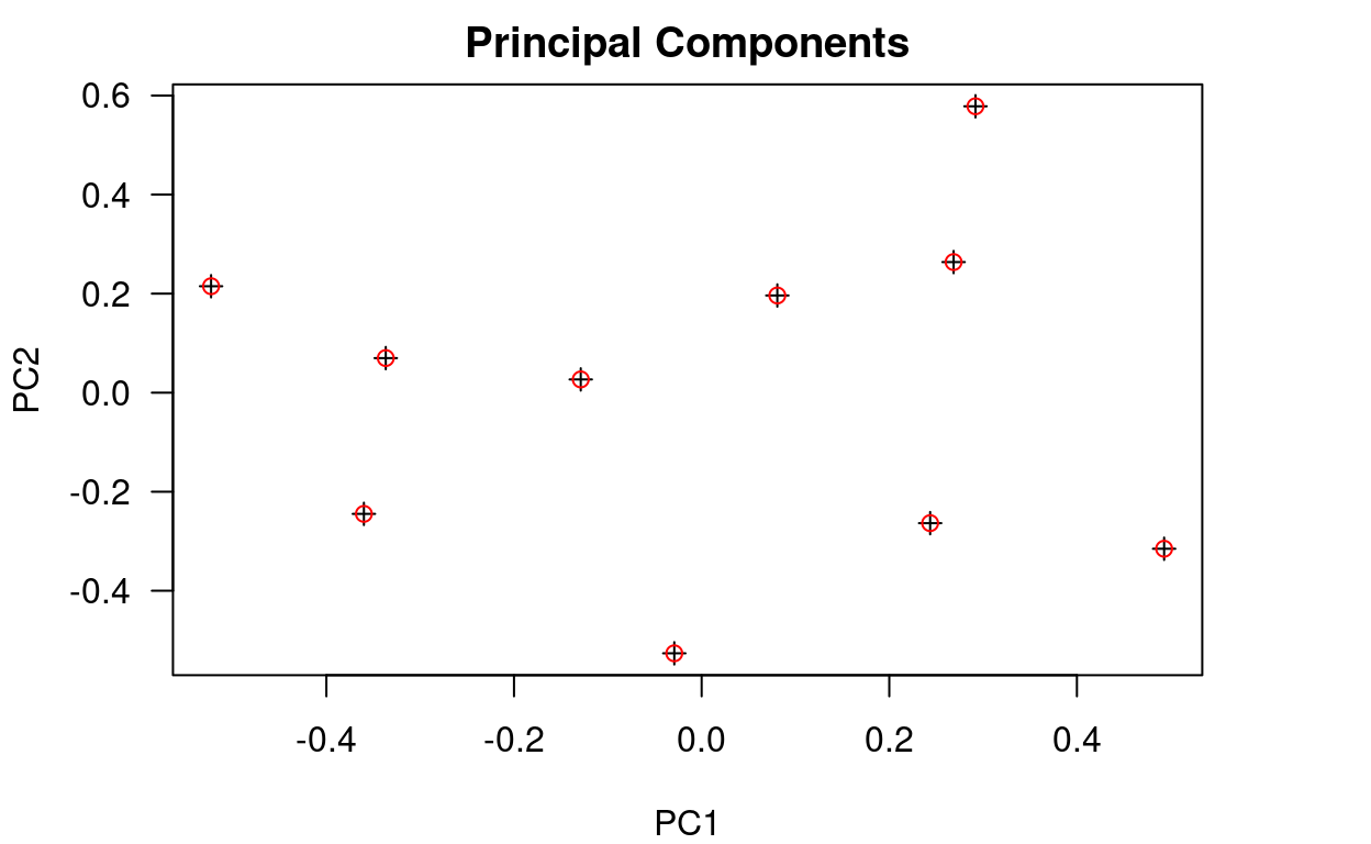

6. Choose principal axes

The eigenvalues of \(Kc\) are used to find the proportion of the total variance explained by the components.

totalVar <- sum(Kc.eign$values)
for (t in Kc.eign$values) {
  print(t/totalVar)
}

## [1] 0.9631813
## [1] 0.03681869
## [1] 4.289189e-17
## [1] 1.03107e-17
## [1] 4.674769e-18
## [1] 2.715163e-19
## [1] -3.685304e-18
## [1] -7.481969e-18
## [1] -8.83757e-18
## [1] -1.623554e-17

7. Principal axes

# scale alpha
r <- 2
PCalpha <- Kc.eign$vectors[,1:r]
n <- dim(X)[1]
for (i in 1:r) {
  PCalpha[,i] <- PCalpha[,i] / sqrt((n-1) * Kc.eign$values[i])
}
# Principal axis
PCAxis1 <- t(Xc) %*% PCalpha[,1]
PCAxis2 <- t(Xc) %*% PCalpha[,2]

So we have obtained the same principal axes PCAxis1 and PCAxis2 as C.eigen$vectors

par(oma=c(0, 0, 0, 0), mar = c(4, 4.1, 2, 4), las="1", xpd=TRUE)
PCAStandard <- matrix(NA, nrow = 2,  ncol = 2) 
PCAStandard[1,] <- C.eigen$vectors[,1]
PCAStandard[2,] <- C.eigen$vectors[,2]
plot(PCAStandard, pch=3, xlab = "PC1", ylab = "PC2", main = "Principal Axes")
# up to a factor -1
PCAKernel <- matrix(NA, nrow = 2,  ncol = 2)
PCAKernel[1,] <- PCAxis1
PCAKernel[2,] <- -PCAxis2
points(PCAKernel, col='red')
legend("topright", inset = c(-0.5, 0), legend = c("Standard","Kernel"), pch = c(3,1), 
       col = c(1,2), title = "Method")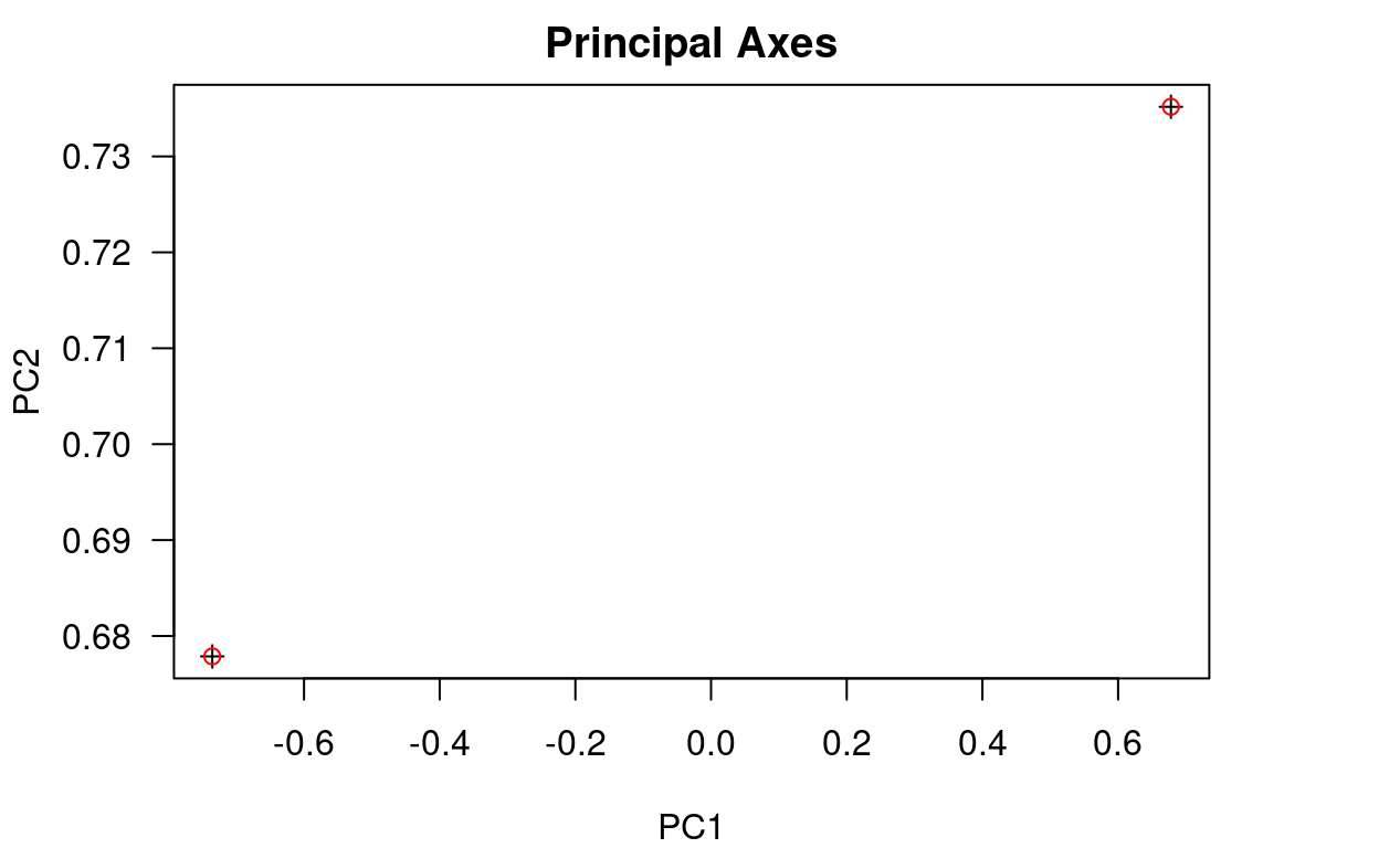

Validation

library(kernlab)

## 
## Attaching package: 'kernlab'

## The following objects are masked from 'package:pracma':
## 
##     cross, eig, size

## The following object is masked from 'package:ggplot2':
## 
##     alpha

# initialize kernel function
linK <- vanilladot()
kpc <- kpca(Xc, kernel=linK)
# return principal component vectors
pcv(kpc)

##              [,1]       [,2]
##  [1,]  0.22656759  1.2535653
##  [2,] -0.48642101 -1.0226454
##  [3,]  0.27150712 -2.7515536
##  [4,]  0.07503555 -0.9335934
##  [5,]  0.45857001  1.4996976
##  [6,]  0.24982141 -1.2547618
##  [7,] -0.02712053  2.5042249
##  [8,] -0.31320326 -0.3322786
##  [9,] -0.11986791 -0.1271683
## [10,] -0.33488896  1.1645133

# return eigenvalues
eig(kpc)

##     Comp.1     Comp.2 
## 1.15562494 0.04417506

# return the data projected on kernel pc space
rotated(kpc)

##             [,1]        [,2]
##  [1,]  2.6182716  0.55376322
##  [2,] -5.6212026 -0.45175422
##  [3,]  3.1376040 -1.21550044
##  [4,]  0.8671295 -0.41241542
##  [5,]  5.2993494  0.66249230
##  [6,]  2.8869986 -0.55429176
##  [7,] -0.3134116  1.10624283
##  [8,] -3.6194550 -0.14678426
##  [9,] -1.3852235 -0.05617669
## [10,] -3.8700604  0.51442443

# returns the kernel used
kernelf(kpc)

## Linear (vanilla) kernel function.

Due to the small size of the toy data matrix, \(n\) and \(n-1\) makes a difference. In standard PCA prcomp, the factor is \(1/(n-1)\). In kpca in kernlab, the factor is \(1/n\).

S <- (t(Xc) %*% Xc)/n
S.eign <- eigen(S)
V <- S.eign$vectors
m <- dim(V)[2]
for (i in 1:m) {
  V[,i] = V[,i] / sqrt(n*S.eign$values[i])
}
# normalized principal components, rotated shows unnormalized PC
Z <- Xc %*% V

S.eign$values

## [1] 1.15562494 0.04417506

eig(kpc)

##     Comp.1     Comp.2 
## 1.15562494 0.04417506

Z

##              [,1]        [,2]
##  [1,]  0.24356016 -0.26347265
##  [2,] -0.52290258  0.21493822
##  [3,]  0.29187014  0.57831779
##  [4,]  0.08066321  0.19622138
##  [5,]  0.49296275 -0.31520440
##  [6,]  0.26855801  0.26372412
##  [7,] -0.02915456 -0.52633457
##  [8,] -0.33669350  0.06983786
##  [9,] -0.12885800  0.02672807
## [10,] -0.36000563 -0.24475581

# rotated, principal components non-scaled to unit norm
z <- rotated(kpc)[, 1]  
# recover principal components
z/sqrt(sum(z^2))

##  [1]  0.24356016 -0.52290258  0.29187014  0.08066321  0.49296275  0.26855801
##  [7] -0.02915456 -0.33669350 -0.12885800 -0.36000563

# recover principal axis
pc1 <- t(Xc) %*% pcv(kpc)[, 1]
pc1 <- pc1 / sqrt(sum(pc1^2))
pc1

##           [,1]
## [1,] 0.6778734
## [2,] 0.7351787

S.eign$vectors[,1]

## [1] 0.6778734 0.7351787